Bin Sui (隋斌), She-hua Huang (黃社華)

State Key Laboratory of Water Resources and Hydropower Engineering Science, Wuhan University, Wuhan 430072, China, E-mail: bins@whu.edu.cn

Numerical analysis of flow separation zone in a confluent meander bend channel*

Bin Sui (隋斌), She-hua Huang (黃社華)

State Key Laboratory of Water Resources and Hydropower Engineering Science, Wuhan University, Wuhan 430072, China, E-mail: bins@whu.edu.cn

The flow pattern in the confluent meander bend channel under the conditions of different discharge ratios and junction angles is numerically simulated by means of the large eddy simulation (LES), and the characteristics of the flow separation zone are analyzed. Numerical results are well validated by experimental data with a good agreement. Analysis of the vertical confinement shows that the turbulence within the separation zone can be characterized as quasi-2-D. Details of the separation zone characteristics are revealed as shown by mean velocity isolines. According to the analysis of numerical results, the length and the width of the separation zone generally increase with the increase of the discharge ratio and the junction angle. However, the width of the separation zone keeps substantially constant when the junction angle increases from 60oto90o. The dimensionless shape of the separation zone is nearly the same for three discharge ratios and three junction angles. The formulas of the relative width and the relative length of the separation zone are obtained by means of the polynomial fit method.

Large eddy simulation (LES), separation zone, discharge ratio, junction angle, quasi-2-D

Introduction

A river confluence can be divided into six zones according to the flow dynamics: the flow stagnation zone, the flow deflection zone, the flow separation zone, the maximum velocity zone, the distinct shear layer zone and the flow recovery zone. The sizes of these zones are controlled by the discharge ratio and the junction angle between the confluent streams. The characteristics of the flow separation zones and the shear layers were analyzed by experimental studies and numerical modeling of confluent straight channels. The dimension of the separation zone in the open channel junction becomes larger when the discharge ratio and the junction angle increase[1-3], and the size of the separation zone decreases when the dredging depth increases[4]. Mao et al.[5]and Creelle et al.[6]studied flows in channel junctions and, in particular,focused on the changes of the dimensions of the separation zone for different junction angles and discharge ratios. They pointed out that the separation zone disappears near the riverbed and the shape of the separation zone is never changed for different discharge ratios or junction angles. However, the above studies mainly focused on straight channels, and only a few on separation zones in confluences of a meandering channel[7-10]. The area of a separation zone in the confluence of downstream rivers is a very important factor because it controls the width of the confluent flows of both the main stream and the tributary with a direct influence on the expected flow velocity and bed shear. Also, in the separation zone one has a recirculating flow in an area of reduced pressure and sediment deposition with a number of consequences, including hydraulic geometry and river roughness[11-13].

As mentioned above, there were several studies concerning the properties of the flow separation zone in the river confluence especially for straight channel confluent flows. However, there still lacks a complete quantitative relationship between the width and the length of the separation zone for various discharge ratios and junction angles. Therefore, this papernumerically explores the characteristics of the separation zone of a more complicated confluence of meander bend channels. More details of the flow separation zone are revealed for the prediction of the sediment transport and the river bed evolution.

1. Numerical model setup

Figure 1 shows the numerical model (with thez-direction pointing upwards) that consists of a 1 m wide main channel and 0.3 m wide tributary channel. The main channel consists of a 4 m long straight inlet, ao

180 reach, and a 4 m long straight outlet. The centerline radius of the curved reach is 2 m. The inlet part and the outlet part of the main channel are parallel. The curved segment has a rectangular cross-section. The intersection at the confluence between the tributary and the main channel is located at ao

90cross-section (CS4). The tributary channel is a straight rectangular flume of 3.5 m long. Takeo90 as the junction angle between the tributary and the main channel, for example. The gradient of the straight main channel is 1/2000, and the average gradient of the curved segment and the tributary are 1/1250 and 1/1000, respectively.

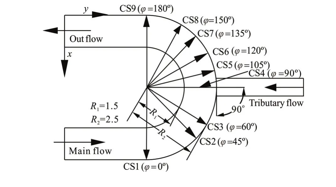
Fig.1 Conceptual model of the confluent meander bend (junction angle is90o)

The discharge from the main channel is denoted asQM(QM=30 L/s) and the discharge from the tributary channel is denoted asQT. Three different discharge ratios (λ=QT/QM=0.1, 0.3, 0.6) and three different junction angles (α=30o, 60oand 90o) are considered in the simulation, with the simulation result of theo

90 junction angle and the simulation result of the discharge ratio of 0.6 as the references. The simulation of the 3-D flow through the meander bend in the numerical model is performed using Openfoam[14]with the large-eddy simulation (LES). The subgrid scales in the LES are captured with a Smagorinsky closure model.

A structured hexahedral mesh is adopted in the model. The grid has a greater density in the junction area, because the hydraulic elements in this region have are relatively larger variations than those at other locations, and a boundary layer grid is used near the boundaries. A 3-D structured grid system with 6.6×106elements is generated with the grid generator GAMBIT.

The numerical model employed in this study is based on the 3-D LES turbulence model. In the LES simulation, the filtered velocity and pressure fields are solved, whereas the influence of the filtered smallscale features on larger eddies is modeled through a subgrid stress (SGS) model. The equations for the LES method are as follows:

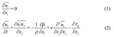
whereis the filtered large eddy velocity, andτijis the modeled SGS that accounts for the influence of the sub-grid eddies on the large eddies. The SGS model is as follows:

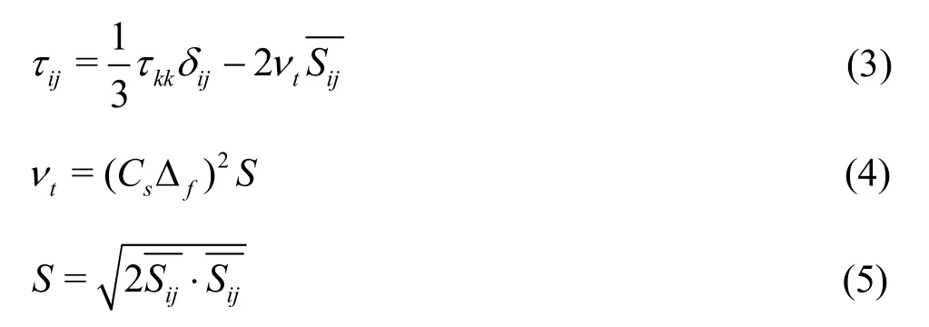
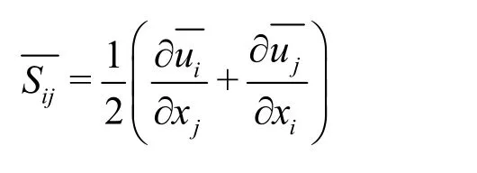
whereis the filtered strain rate tensor, defined as

The inflow conditions of the velocity and the height of the inlet are obtained by experimental measurements[15]. For the inlet boundary, the flow discharge and the velocity of the main channel are specified. The pressure is chosen to have a zero normal gradient for consistency with the velocity condition. The outlet boundary is set to have a zero gradient. The free surface is described by the rigid-lid approximation (using the measured water surface data). The finite volume method (FVM) is used for the discretization of the Navier-Stokes equations, and the pimpleFoam algorithm is used for the velocity and pressure coupling. The central difference scheme is adopted for the diffusion terms of the governing equation, and the convection term is solved by a first order upwind scheme.

2. Model validation

Experiment data are used to validate the numerical model of the confluent meander bend flow. Figures 2, 3 and 4 display the streamwise velocity (Va)variations against the water depth(d) at CS3 (φ=60o)and CS6(φ=120o) cross-section in the bend channel,where the discharge ratio isλ=0.6 and the junction angle isα=30o, 60oand 90o, respectively (The dashed line representsY-axis). Figures 5, 6 and 7 display the flow velocity vectors on the water surface for various discharge ratios and junction angles, where the junction angle isα=90oand the discharge ratio isλ=0.6, respectively. Figures 5, 6, 7(a2) and 7(b2) show the same trends for the velocity vectors. But as shown in Fig.7(a1) (LES data), the small area of the separation zone appears along the outer bank at the downstream of the junction, while in the experiment data (Fig.7(b1)) this separation zone does not exist for the case of the tributary entry angle ofo30. This is mainly due to the fact that the small separation zone cannot be captured by the experiment measurement.

In this way, the reliability of the numerical model is validated. The experiment data agree well with the calculated results and give the same trends of the flow velocity, which ensures that the numerical results are reasonable and reliable.

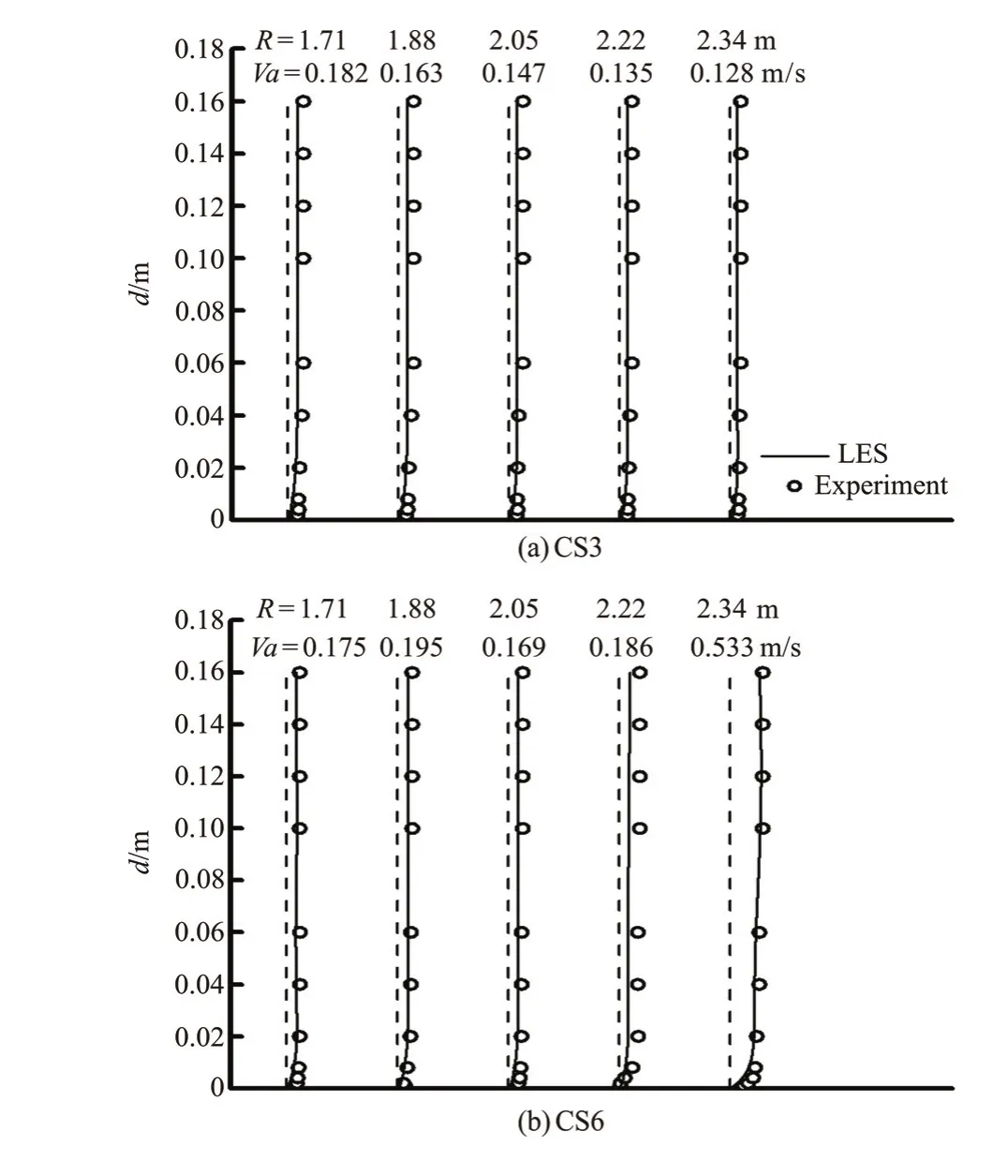
Fig.2 Comparison of numerical results and model test data for a streamwise velocity distribution in two cross sections

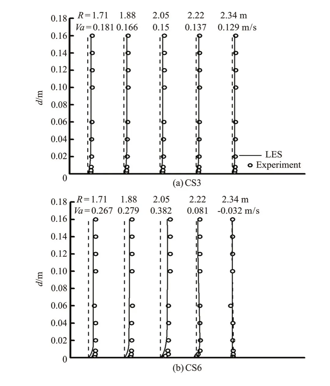
Fig.3 Comparison of numerical results and model test data for a streamwise velocity distribution in two cross sections

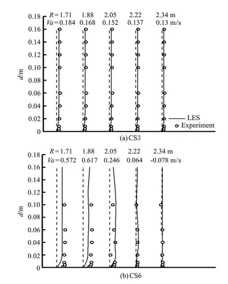
Fig.4 Comparison of numerical results and model test data for a streamwise velocity distribution in two cross sections

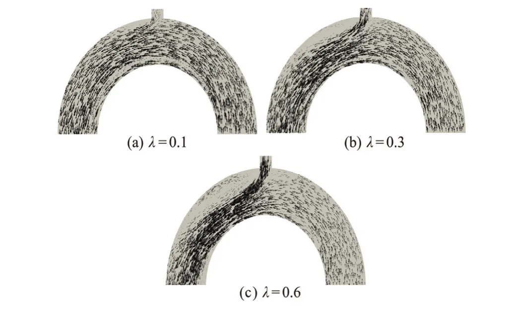
Fig.5 Comparison of flow velocity vectors on the water surface for various discharge ratios (LES data)

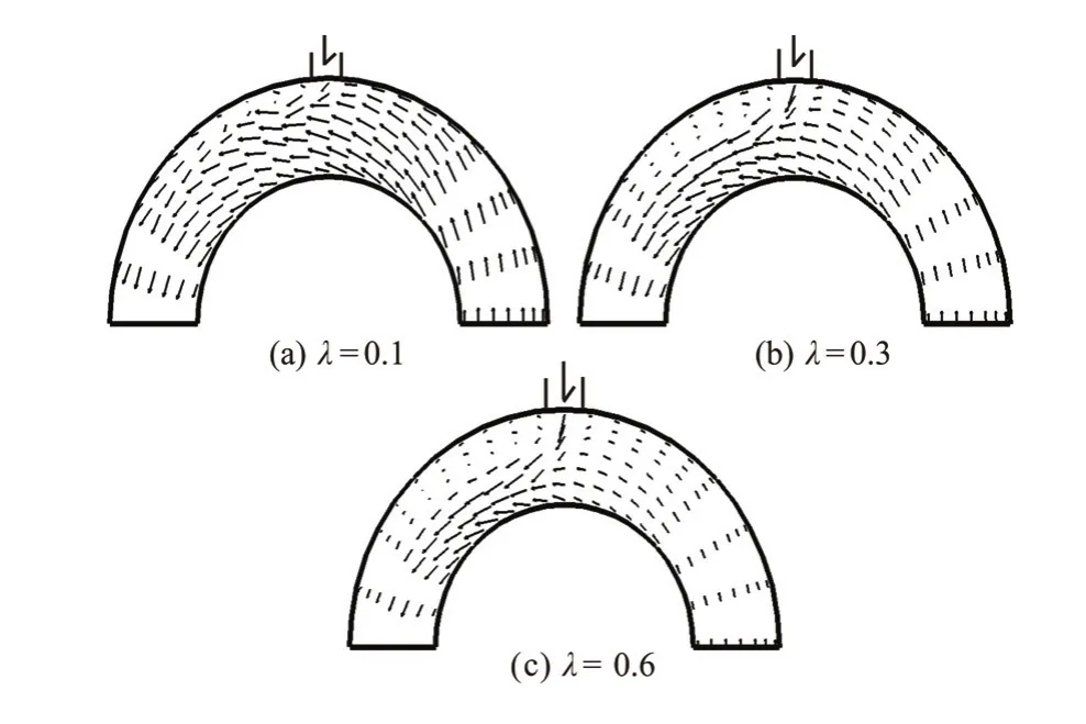
Fig. 6 Comparison of flow velocity vectors on the water surface for various discharge ratios (Experiment data)

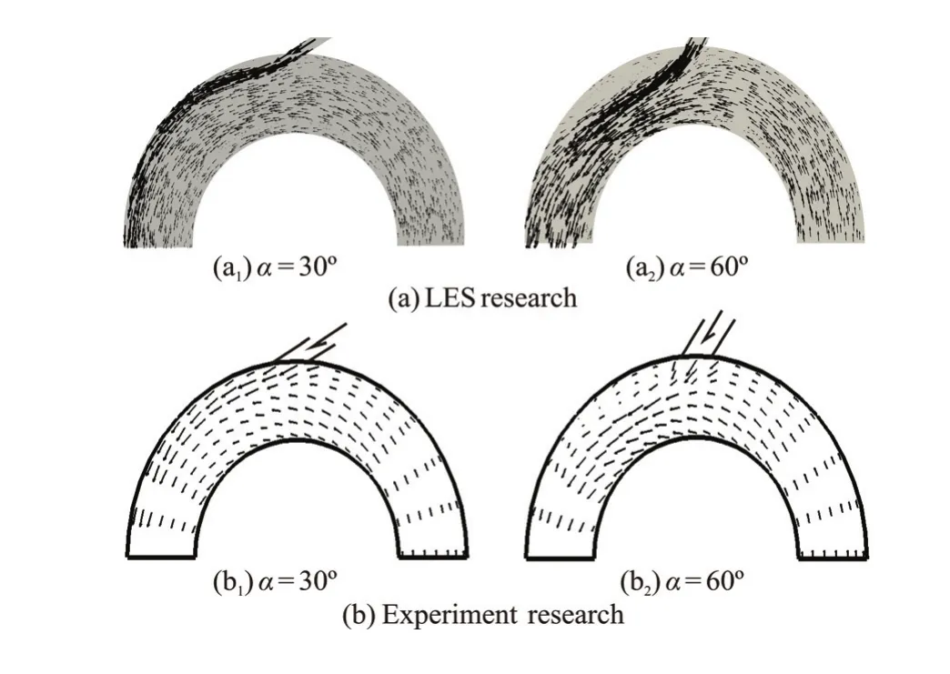
Fig.7 Comparison of flow velocity vectors on the water surface for various junction angles

3. Analysis of simulation results

3.1 Influence of vertical confinement

The flow structure is measured by computing the correlation product between the velocity fields on seven horizontal slices: the lower slices SL1=0.01m, SL2=0.03m and SL3=0.06 m above the bottom, the middle slice at the half depth SL4=0.09 m, and the upper slices SL5=0.12 m, SL6=0.16 m, SL7=0.18m above the bottom. The correlation product is given by[16]

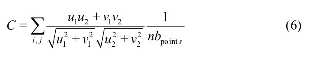
where(u1,v1),(u2,v2)are the velocity components given at each point of the mesh grid on two different slices, andi,jrepresent the mesh grids constituted by

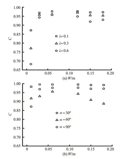
Fig.8 Correlation product

Figure 8(a) shows the correlation products forλ=0.1, 0.3 and 0.6, and Fig.8(b) shows the correlation products forα=30o, 60oand 90o. The correlation product is computed based on the values provided by the lower and middle slices and by the upper and middle slices. If the correlation product is equal to 1, the velocity fields are totally identical between(u1,v1) and(u2,v2). For the three discharge ratios, the value provided by SL1 and SL4 is smaller than the other values, and, with the exception of this value, the correlation product is in the range from 0.90to 0.98. For the three junction angles in Fig.8(b), the correlation product is between 0.85 and 0.98. Although the correlation product is never equal to 1.0, the trend is to approach 1.0, which means that the vertical velocity has little influence on the separation zone flow structures, and the maximum Froude number is 0.147 at downstream of the junction, so the turbulent flows within the separation zone can be characterized as quasi-2-D[17]. Thus we choose the middle slice at the half depth (SL4) to study the characteristics of the flow separation zone.

3.2 Separation zone characteristics

In this paper, the main channel has a meander bend shape, a Cartesian coordinate system is not best suited for this shape but the cylindrical coordinates might easily do the job. To have a clearer picture of the separation zone characteristics in a confluent meander bend channel, we convert the numerical results from a Cartesian to a cylindrical coordinate system. Figure 9(a) shows the streamwise mean velocities of the study domain (from CS4 to CS9) in the Cartesian coordinates (we use the case ofα=90oandλ=0.6 as an example) and Fig.9(b) shows the streamwise mean velocities of the study domain (from CS4 to CS9) in the cylindrical coordinate system.

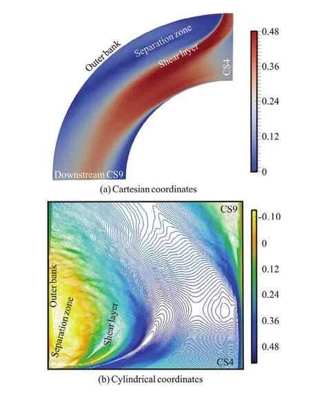
Fig.9 (Color online) Streamwise mean velocities in the study zone

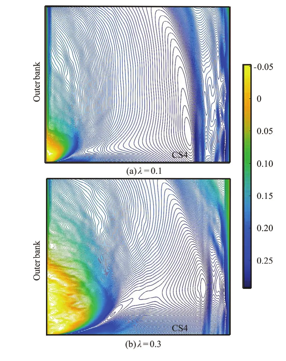
Fig.10 (Color online) Streamwise mean velocities in the study zone

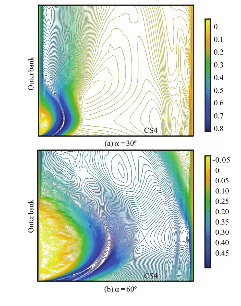
Fig.11 (Color online) Streamwise mean velocities in the study zone

Figure 10 shows the streamwise mean velocity inthe study zone for different discharge ratios, where the junction angle iso90. Figure 11 shows the streamwise mean velocity for different junction angles, where the discharge ratio is 0.6. The separation zone characteristics are usually expressed by the width and the length of the zone. As Figs.9(b), 10, and 11 show, when the discharge ratio and the junction angle increase, the area of the separation zone also increases. Both the width and the length of the separation zone increase.

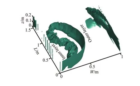
Fig.12 (a) (Color online) The shape of the shear layer

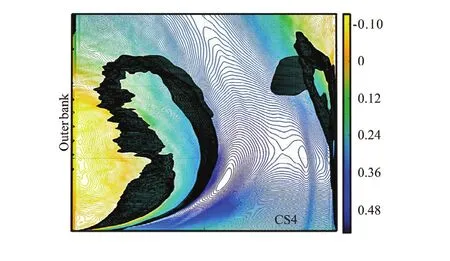
Fig.12(b) (Color online) the streamwise mean velocities and the isosurface of the shear layer

According to the boundary layer theory, the separation zone begins at the point where the flow velocity cannot overcome the adverse pressure gradient, therefore, the velocity at these separation zone border is equal to zero[18]and the zero-velocity isolines is taken as the separation zone border in this paper. Through analysis and comparison, the same phenomenon is found in the shear layer for two other discharge ratios and junction angles, so we may analyze the case of the discharge ratioλ=0.6 andas an example (Fig.12, whereW,Lrepresents channel width, arc length at downstream of the junction). It was suggested that the shear layer is a 3-D structure[19], consisting of an inner layer (rough surface) and an outer layer (smooth surface). The turbulent structure in the shear layer is related to the turbulence intensities[20]. Thus, the inner layer is rough (Fig.12(a)), which is influenced by the maximum turbulence velocity. As shown in Fig.12(b), the separation zone is seen very clearly. The streamwise velocity plays an important role in the flow structure, so it also has a significant effect on the shape of the separation zone. In this study, a streamwise velocity isoline with a zero mean-velocity represents the border of the separation zone.

Figure 13 shows the area of the separation zone in the study domain for (a) different discharge ratios, and (b) different junction angles. Curves represent borders of the separation zone for different discharge ratios and junction angles, with the horizontal and longitudinal coordinates standing for the channel width and the length of the outer bank, respectively. As the discharge ratio and the junction angle increase, the length and the width of the separation zone increase with their shape maintaining unchanged. When the junction angle is gradually increased from 60oto 90o, as Fig.13(b) shows, the separation zone has a nearly equal width, and the length of the separation zone increases over a small range.

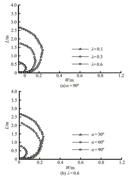
Fig.13 Separation zone in the study domain

To demonstrate that the shape of the separation zone changes with different discharge ratios and junction angles, the dimensionless values are used instead of the original values (Fig.14).

To make the variables dimensionless, the following relation is used

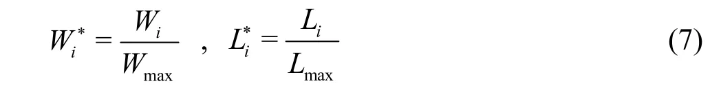
whereWiandLiare the length and the width of the separation zone, respectively.

Figure 14 shows that when the junction angle is fixed, the dimensionless curves of the separation zone for different discharge ratios are nearly the same. And as the discharge ratio is fixed, the dimensionless curves of the separation zone for different junction angles are also nearly the same.

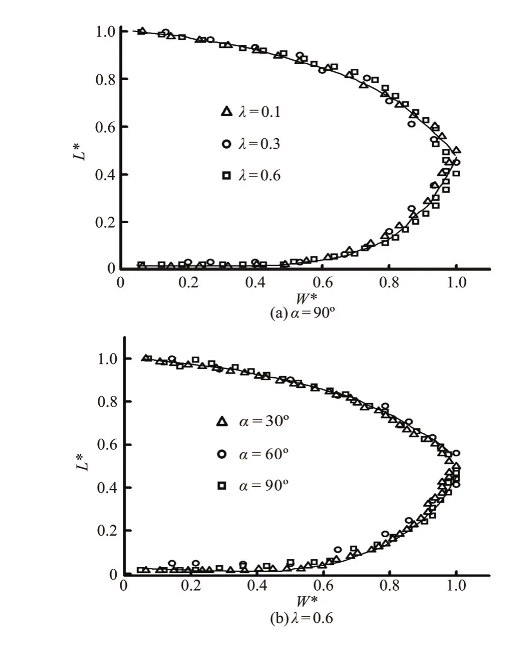
Fig.14 Separation zone with dimensionless values

To better illustrate the characteristics of the separation zones, we consider the cases when the junction angle isα=90o, the discharge ratios areλ=0.1,λ=0.3 andλ=0.6, and the relative width can be described by a polynomial fitting as:

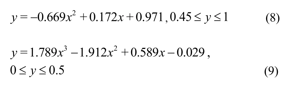
wherexis a relative width, andyis a relative length.

When the discharge ratio isλ=0.6, the junction angles areα=30o, 60oand 90o, and the relative width can be described by a polynomial fit as:

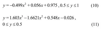
wherexis the relative width, andyis the relative length.

4. Conclusions

This paper investigates the flow structures in a confluent meander bend channel using a 3-D numerical model. According to the analysis, the influence of the vertical confinement and the turbulent structures within the separation zone can be characterized as quasi-2-D. To illustrate the detailed characteristics of the separation zone in a confluent meander bend channel, the numerical results are converted from a Cartesian to a cylindrical coordinate system. The following research results are obtained numerically:

Based on the shear layer boundary theory, the shape of the separation zone is successfully visualized by taking the zero-velocity is oline as the separation zone border.

The length and the width of the separation zone is found to increase with the increase of discharge ratios and junction angles, but when the discharge ratio isλ=0.6 and the junction angle increases from 60oto 90o, the width of the separation zone hardly changes and the length of the separation zone only increases over a small range.

The shape of the separation zone is never changed for different discharge ratios or junction angles according to the dimensionless analysis of the numerical data. Based on the dimensionless values, the functional relationships between the relative width and length of the separation zone are proposed for the confluent meander bend channel flow.

[1] Geberemariam T. K. Numerical analysis of stormwater flow conditions and separation zone at open-channel junctions [J].Journal of Irrigation and Drainage Engineering, 2016. 143(1): 05016009.

[2] Rooniyan F. The effect of confluence angle on the flow pattern at a rectangular open-channel [J].Engineering Technology and Applied Science Research, 2013, 4(1): 576-580.

[3] Yang F. C., Chen X. P. Numerical simulation of twodimensional viscous flows using combined finite elementimmersed boundary method [J].Journal of Hydrodynamics, 2015, 27(5):658-667.

[4] Sik C. H., Mo S. J. An analysis on the characteristics ofseparation zone due to a bed discordance at confluence [J].Journal of Korea Water Resources Association, 2015, 48(8): 625-634.

[5] Mao Z. Y., Zhao S. W., Zhang L. Separation zone of open-channel junction [J].Advances in water science, 2005, 16(1): 7-12(in Chinese).

[6] Creelles S., Mulder T. D., Schindfessel L. et al. Influence of hydraulic resistance on flow features in an open channel confluence [J].Iahr Europe Congress, 2014, 45(2): 527-535.

[7] Roberts M. V. T. Flow dynamics at open channel confluent-meander bends [D]. Doctoral Thesis, Leeds, UK: University of Leeds, 2004.

[8] Wang X. K., Zhou S. F., Ye L. et al. Numerical simulation of confluence flow structure between Jialing River and Yangtze River [J].Advances in water science, 2015, 26(3): 372-373(in Chinese).

[9] Goudarzizadeh R., Jahromi S. H. M., Hedayat N. Simulation of 3D flow using numerical model at open-channel confluences [J].World Academy of Science, Engineering and Technology, 2010, 4(11): 1437-1442.

[10] Riley J. D., Rhoads B. L. Flow structure and channel morphology at a natural confluent meander bend [J].Geomorphology, 2012, 163: 84-98.

[11] Artt D. W. An experimental investigation of film cooling, with particular reference to the injection region [D]. Doctoral Thesis, Belfast, UK: Queen’s University Belfast, 1970.

[12] Huai W., Xue W., Qian Z. Large-eddy simulation of turbulent rectangular open-channel flow with an emergent rigid vegetation patch [J].Advances in Water Resources, 2015, 80: 30-42.

[13] Liu S. H., Cao B. Hybrid simulation of the hydraulic characteristics at river and lake confluence [J].Journal of Hydrodynamics, 2011, 23(1): 105-113.

[14] OpenCFD. OpenFOAM: The open source computational fluid dynamic (CFD) toolbox [EB/OL]. http://www.OpenFoam.org 2005, 2006.

[15] Gao Y., Huang S. H., Li Q. Experimental research on velocity distribution along depth at junction of bend stream with branch afflux [J].Water Resources and Power, 2012, 30(7): 90-93.

[16] Sous D., Bonneton N., Sommeria J. Turbulent vortex dipoles in a shallow water layer [J].Physics of Fluids, 2004, 16(8): 2886-2898.

[17] Constantinescu G., Miyawaki S., Rhoads B. et al. Structure of turbulent flow at a river confluence with momentum and velocity ratios close to 1: Insight provided by an eddy-resolving numerical simulation [J].Water Resources Research, 2011, 47(5): W05507.

[18] Yuan Q. Y., Wang X. Y., Lu W. Z. et al. Experimental study on characteristics of separation zone in confluence zones in rivers [J].Journal of Hydrologic Engineering, 2009, 14(2): 166-171.

[19] Amir M., Castro I. P. Turbulence in rough-wall boundary layers: Universality issues [J].Experiments in fluids, 2011, 51(2): 313-326.

[20] Melnick M. B., Thurow B. S. Comparison of large-scale three-dimensional features in zero-and adverse-pressuregradient turbulent boundary layers [J].AIAA Journal, 2015, 53(12): 3686-3699.

(Received February 27, 2016, Revised March 2, 2017)

* Project supported by the Key Program of National Natural Science Foundation of China (Grant No. 51439007).

Biography:Bin Sui (1985-), Female, Ph. D.

She-hua Huang,

E-mail: hshh2@126.com