Hu Zhaoping,Zhang Chao(College of Sciences,ShanghaiUniversity,Shanghai200444,China)

Linearizability conditions for 1 ∶-5 Lotka-Volterra two-dimensional complex quartic systems

Hu Zhaoping?,Zhang Chao
(College of Sciences,ShanghaiUniversity,Shanghai200444,China)

In thispaperwe investigate the linearizability problem forthe planarLotka–Volterra complex quartic systems which are 1:?5 linear systems perturbed by homogeneous polynomials of degree 4,that is to say,we consider systems of the form˙x=x(1????), ˙y=?y(5????The necessary and sufficient conditions for the linearizability ofthis system are found.

polynomialsystems;linearization;invariantcurve;cofactor

2010 MSC:34C41,34C04

1 Introduction

Consider a real planar analytic differential system with an isolated singular point at the origin,at which the eigenvaluesofthe linearpartare non-zero pure imaginary numbers.By analytic change ofcoordinatesand a constanttime rescaling the system takes the form

By the Poincar′e–Lyapunov theorem,system(1)has a center at the origin if and only if there is a first integralu,v)=u2+v2+···(see for instance[1]and the references therein).

If the origin is a center,then the problem thatarises is to determine when the period of the solutions near the origin is constant.A center with such a property is called an isochronous center.By the isochronous center theorem of Poincar′e and Lyapunov,the centerof(1)is isochronous if and only if itis linearizable.Hence,the isochronicity problem is equivalent to the linearizability problem.Furthermore,it can be generalized to the case of complex systems as follows.Introducing a complex structure on phase plane(u,v)by setting x=u+iv,y=ˉx=u?iv, aftera change oftime idt=dτand rewriting t instead ofτ,system(1)becomesa system oftwo complex differential equations of the form

The origin is the 1:?1 resonantsingularpointofsystem(2).

The nextnaturalgeneralization of the resultabove is to consider the case ofan analytic vectorfield on C2with a p:?q resonantelementary singularpointatthe origin,thatis,a system ofthe form

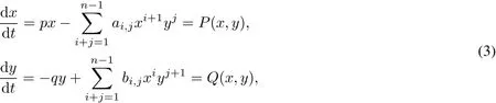
where p,q∈N and GCD(p,q)=1.We denote the coefficients by

We know that

Definition 1[2](i)The system(3)is integrable atthe origin ifthere exists an analytic change ofcoordinates

bringing the system(3)to the system

where h(X,Y)=1+O(X,Y)(XqYp=xqyp+h.o.t.is then a firstintegralof the type introduced by Dulac).The definition is also valid forthe case pq=0.

Moreover,the system(3)is integrable atthe origin ifitadmits a firstintegralofthe form

(ii)The system(3)is linearizable atthe origin ifthere exists an analytic change ofcoordinates

bringing the system(3)to the system

The linearizability problem for the complex system(2)is a generalization of the linearizability(isochronicity) problem forthe realsystem(1).Severalmethods have been developed to compute the necessary conditions to have an isochronous center,see[3–6]and references therein.However,There are only a few families of polynomial differentialsystems in which a complete classification ofthe linearizability(isochronicity)is known,see forinstance [7–9].

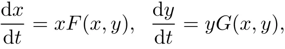
Therefore,more works focused on the integrability and linearizability for the following planar polynomial systems,

System(8)has two invariantlines passing through the origin,and we callita Lotka-Volterra system.The differential equations modeling the interaction of the two species have been studied extensively by realsystems of the form

also known as Kolmogonov systems.

Even in the case ofquadratic nonlinearities,itis already necessary to restrictthe class ofsystems underconsideration.Forexample,fora 1:?q resonantquadratic system,indeed,complete results aboutintegrability are known only for Lotka–Volterra systems:

Theorem 1[2]For q∈N/{1}the Lotka?Volterra system˙x=x(1+A1x+B1y),˙y=y(?q+A2x+B2y) has a resonantcenteratthe origin ifand only if

Recently,the integrability and linearizability problem for some Lotka-Volterra system having homogeneous nonlinearities with higherdegree are considered.The 1:?q cubic Lotka–Volterra system was studied in[10–11]; linearizability of the 1:?1 quartic Lotka–Volterra system was considered in[12];integrability of the 1:?1 quintic Lotka–Volterra system was considered in[13–14].

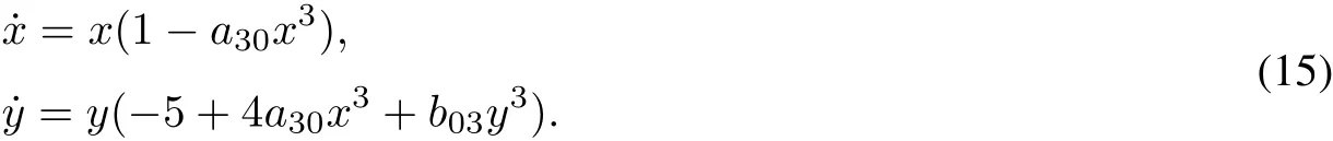
In this paper we study the linearizability problem for a class of quartic systems with 1:?5 resonantsaddle, namely the corresponding completely quartic homogeneous Kolmogonov system,

In the work we obtain necessary and sufficientconditions for(9)to be linearizable atthe origin.

2 Preliminaries

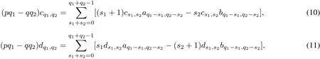
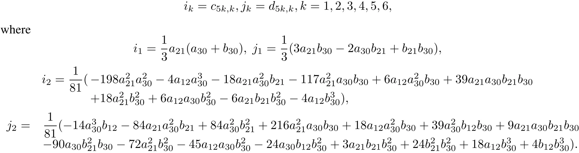
In this section,we briefly describe the generalapproach to study the integrability and linearizability problem for the polynomialsystem(3).The firststep is the calculation of the so-called linearizability quantities,which are polynomials ofthe coefficients ai,jand bi,jofsystem(3).Taking derivatives with respectto t in both parts of each of the equalities in(7)and equating coefficients of the terms xq1+1yq2for the first equation and xq1yq2+1for the second equation we obtain the recurrence formulaewhere s1,s2≥?1,q1,q2≥?1,q1+q2≥1,c1,?1=c?1,1=d1,?1=d?1,1=0,c0,0=d0,0=1 and we set ap,q=aq,p=0 if p+q＜1.Hence,we compute the cq1,q2and dq1,q2of the formalchange of variables(6) step by step using the fomulae(10)and(11).In the case pq1=qq2=kpq the coefficients cqk,pkand dqk,pkcan be chosen arbitrarily(we set cqk,pk=dqk,pk=0).The system is linearizable if and only if the quantities on the right-hand side of(10)and(11)are equalto zero for all pq1=qq2=kpq,k∈N.In case pq1=qq2=kpq we denote the polynomials on the right-hand side of(10)by ikand on the right-hand side of(11)by?jk,calling them the k?th linearizability quantities.Hence,system(3)with the given coefficient(A,B)is linearizable if,and only if, ik(A,B)=jk(A,B)=0 for all k∈N.

In the space of the parameters of a given family of systems(3)the set of all linearizable systems is an affine variety V of the ideal＜i1,j1,i2,j2,···＞.We recall that the variety of a given set of polynomials F=＜f1,f2,···,fs＞is the set of common zeros of the polynomials f1,f2,···,fsand it is denoted by V(F). Denote by Ikthe idealgenerated by the first k pairs ofthe linearizability quantities,

By the Hilbertbasis theorem there exists N∈N such that V=V(＜i1,j1,i2,j2,···＞)is equalto the variety of the ideal IN,V=V(IN).However,the theorem does notgive a constructive procedure to find N.In practice,N is taken such that

Subsequently,the minimal associated primes of the ideal are computed.The computational tool we used is the routine minAssGTZ of the computeralgebra system SINGULAR which computes the decomposition using the method described in[1].For each componentone tries to find the linearizing transformation(6).

The mostpowerfulmethod to find linearizing transformationsis the so-called Darboux linearization,see[1–2]. A smooth function f(x,y)satisfying

is called a Darboux factorofsystem(3)and the polynomial k(x,y)is called the cofactor.

To constructa Darboux firstintegralfor system(3),we have the following theorem.

Theorem 2[1]Ifthere are Darboux functions f1,f2,···,fmwith the cofactors k1,k2,···,kmsatisfying

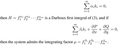
Moreover,if system(3)admits an integrating factor,then the system is integrable and admits a firstintegralof the form(5).

Obviously,a linearizable system(3)should be integrable.The following theorem allows us to constructlinearizing substitutions if sufficiently many Darboux factors are known,and italso provides a method to find linearizing substitutions for integrable system.

Theorem 3[2]The system(3)is linearizable if one of the following situations occurs:

Case I:There exist analytic functions F1(x,y),···,Fm(x,y),K1(x,y),···,Km(x,y)defined in aneighborhood ofthe origin and numbersα,···,α,β,···,β satisfying+=K F and1m?12mii

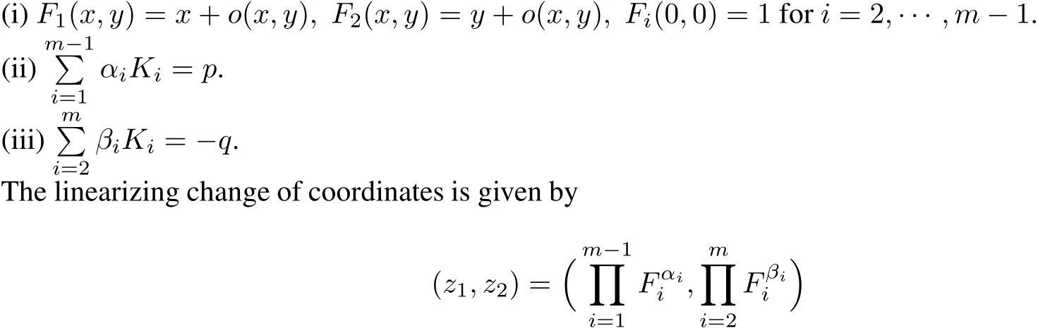
and the system is integrable with firstintegral z

Case II:The system is integrable with first integralΦ(x,y)～and there exist analytic functions F1(x,y),(,K1(x,y),···,Km(x,y)defined in a neighborhood of the origin and numbersα1,···,αmsatisfying+=KiFiand

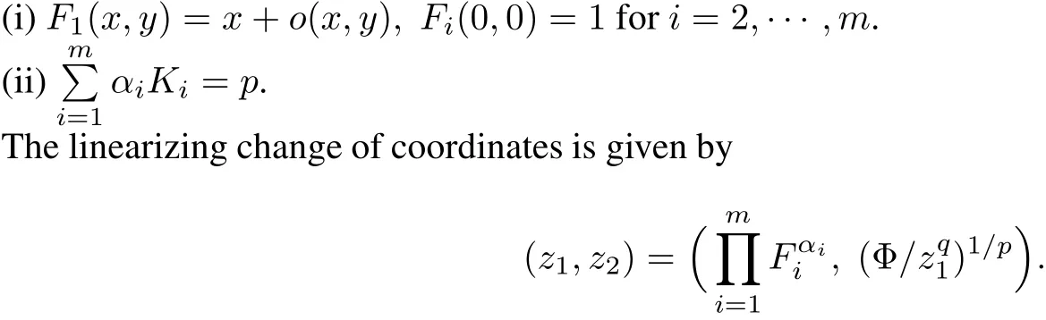
Case III:The system is integrable with first integralΦ(x,y)～xqypand there exist analytic functions F1(x,y)···,Fm(x,y),K1(x,y),···,Km(x,y)defined in a neighborhood of the origin and numbersβ1,···,βmsatisfying+˙=K F andii

In fact,this theorem tells us that,if system(3)is integrable and one of the equations is linearizable,then the other equation should be linearizable too.More details on the Darboux method of integration and linearization can be found in[1].

3 The linearizability conditions

In this section,we willfind the necessary and sufficientconditions for linearizability of system(9).Using a straightforward modification of Mathematica code from[8],we have computed the firstsix pairs of linearizability quantities.The polynomials are too long,so we do notpresentthem here.The interested readercan easily compute them using any available computer algebra system with the algorithms of[1],for instance.Then,we find that V(I4)=V(I3).Using the routine minAssGTZ of the computeralgebra system SINGULAR,we obtain the minimal associated primes of the ideal I3.Finally,foreach componentwe find the linearizing transformation(6).Thus,we obtain the necessary and sufficientconditions for linearizability of system(9)as follows.

Theorem 4 System(9)is linearizable if and only if one of the following conditions holds:

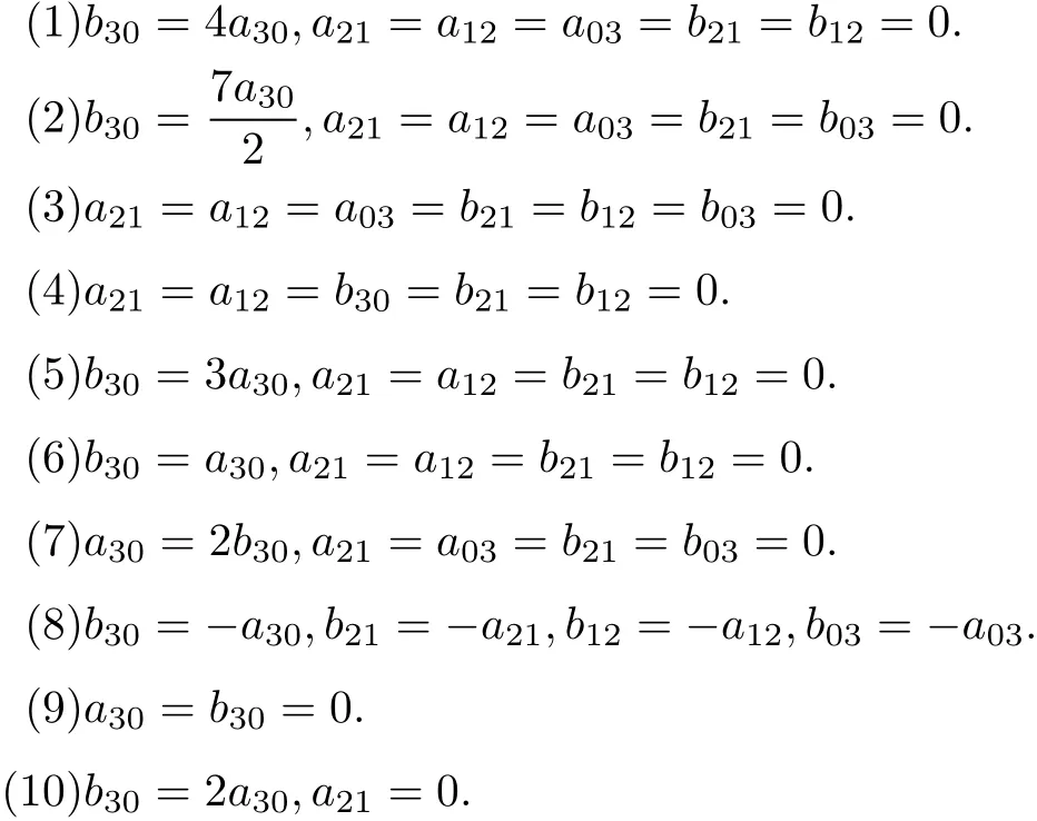
Proof First,according to the definition oflinearizability quantities,we calculate the firstsix groupsoflinearizability quantities,

We now show thatundereach condition the system(9)is linearizable.

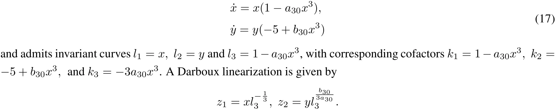
Case 1 In this case,system(9)can be written as

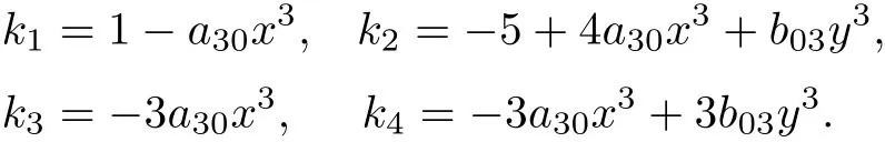
Using the described Darboux integrability approach we have found that the system has the following four algebraic invariantcurves:l1=x,l2=y,l3=1?and l4=1?a30x3?with corresponding cofactors

Case 2 In this case,system(9)takes the form

It has four algebraic invariant curves:l1=x,l2=y,l3=1?a30x3and l4=1?a30x3?2 9b12xy2with corresponding cofactors

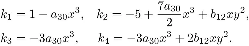
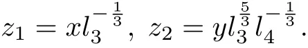
Thus,a Darboux linearization of(16)is given by

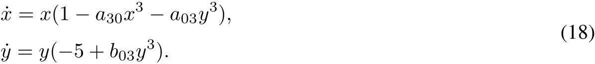
Case 3 In this case,the system(9)has the form

Case 4 In this case,the corresponding system is

Case 5 In this case,system(9)takes the form

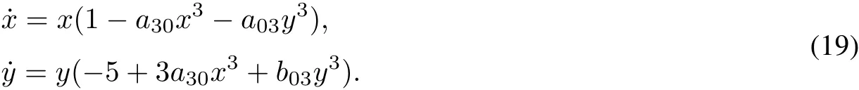
Using the transformations

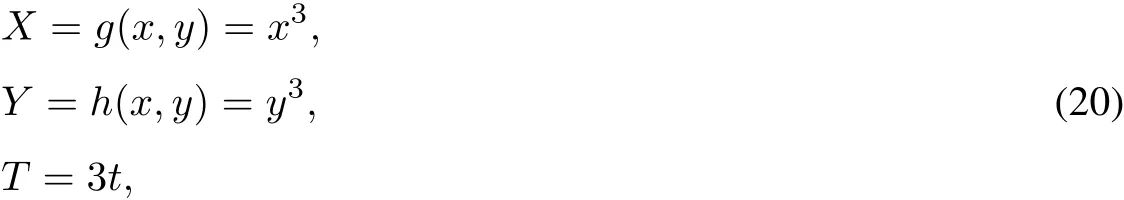
we rewrite system(19)into the form

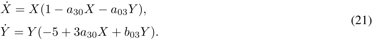
By Theorem 1,system(21)is linearizable.Therefore,system(19)is also linearizable.

Case 6 In this case,system(9)takes the form

Using the transformations(20),we rewrite system(22)into the form

By Theorem 1,system(23)is linearizable.So system(22)is also linearizable.

Case 7 In this case,system(9)takes the form

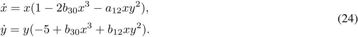
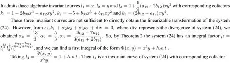
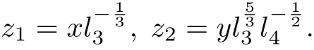
Thus,a Darboux linearization of the system(24)is give by

Thus,a Darboux linearization is given by

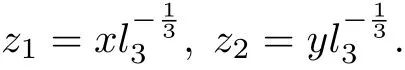
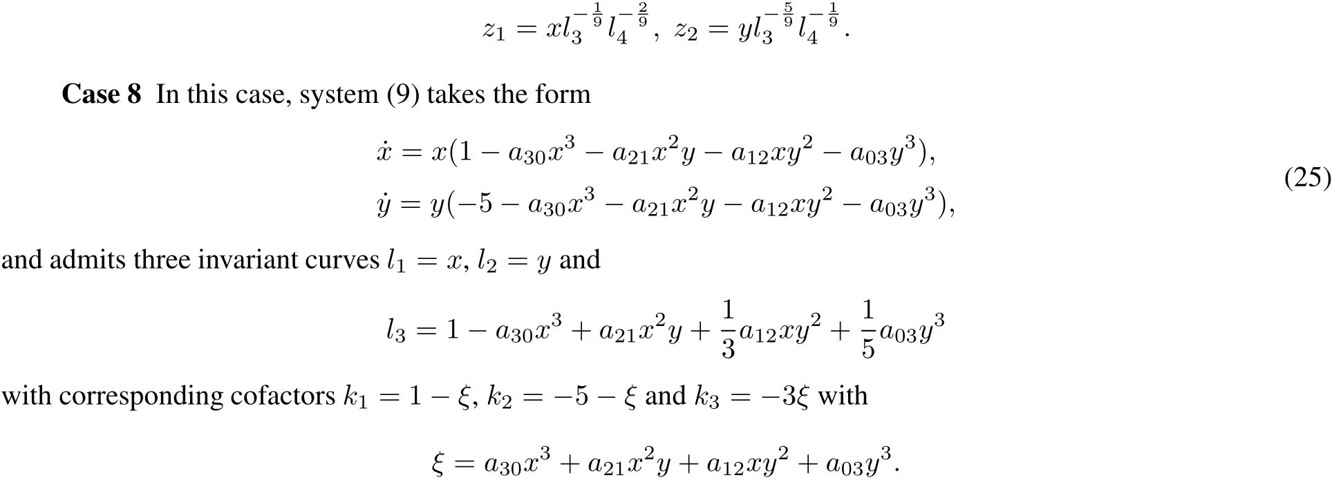
Case 9 In this case,system(9)takes the form

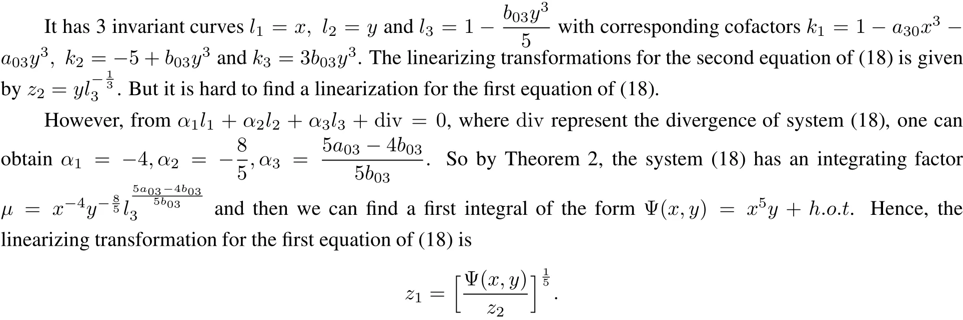
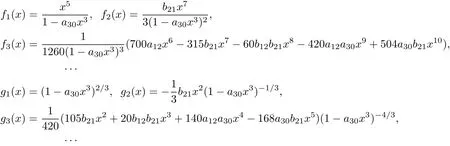
However,itis hard to find more invariantcurve except x and y.Now,we try to prove itby finding formallinearization z1and z2.

Firstly,we look fora Darboux firstintegralof system(26)in the form of a power series

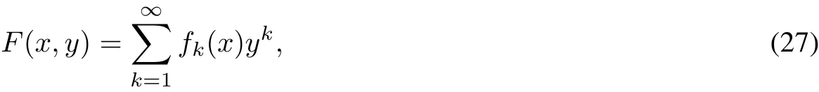
satisfying f1(x)=x5+o(x5).According to˙F=0,the functions fk(x)satisfy the system of equations

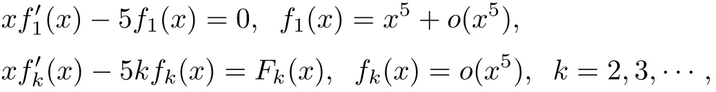
where

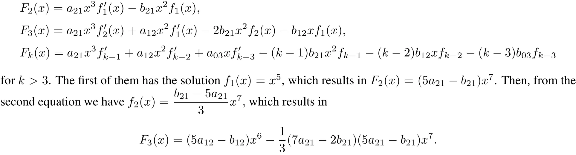
Step by step,we can obtain fk(x)easily.Obviously,fk(x)is a polynomialof degree 2k+3 for any k=1,2,···. Therefore,the system is integrable.

By Theorem 3,we only need to prove thatone of the linearizing transformation z1or z2exists.Now,we look fora linearizable transformation ofthe second equation ofsystem(26)in the form ofa powerseries

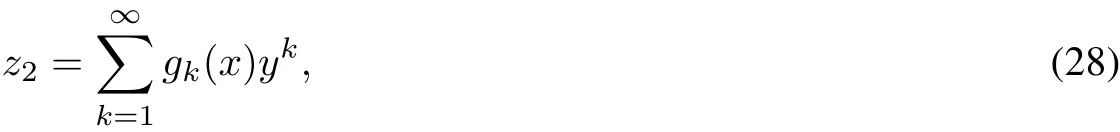
satisfying g1(x)=1+O(x).According to˙z2=?5z2,the functions gk(x)satisfy the system of equations

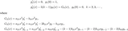
for k＞3.The firstofthem has the solution g1(x)=1,which results in G2(x)=?.Then,from the second equation we have

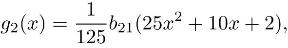
which results in

Step by step,we can obtain gn(x)easily.Obviously,both Gk(x)and gk(x)are polynomials of degree 2(k?1).By Theorem 3 the system is linearizable.

Case 10 In this case,system(9)takes the form

Similarly as in case(9),we look for a firstintegral F(x,y)and a linearizable transformation z2in the form of a powerseries,

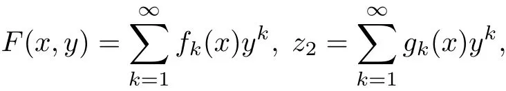
So the functions fk(y)and gk(x)satisfy the system ofequations

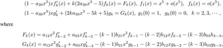
and gj(x)=hj(x)=0 for j≤0.

Step by step,we can obtain from the above equations that

Therefore,by Theorem 3 the system(29)is linearizable.

[1]Romanovski V G,Shafer D S.The center and cyclicity problems:A Computational algebra approach[M].Boston: Birkh¨a user,Boston inc,2009.

[2]Christopher C,Mardeˇs ic P,Rousseau C.Normalizable integrable and linearizable saddle points for complex quadratic systems in C2[J].JDynam Control Syst,2003,9:95-123.

[3]Liu Y,Li J.Theory of values of singular point in complex autonomous differential systems[J].Sci China Ser A,1990, 33(1):10-24.

[4]Zoladek H.The problem ofcenterforresonantsingularpoints ofpolynomialvectorfields[J].JDiff Eqs,1997,137:94-118.

[5]Liu Y,Huang W.A new method to determine isochronous center conditions for polynomial differential systems[J].Bull Sci Math,2003,127(2):133-148.

[6]Lin Y,Li J.The normal form of a planar autonomous system and critical points of the period of closed orbits[J].Acta Math Sin,1993,34:490-501(in Chinese).

[7]Chavarriga J,Gin′e J,Garc′i a IA.Isochronous centers of a linear center perturbed by fourth degree homogeneous polynomial[J].BullSciMath,1999,123:77-96.

[8]Romanovski V G,Robnik M.The centre and isochronicity problems for some cubic systems[J].J Phys A,Math Gen, 2001,34(47):10267-10292.

[9]Chen X,Romanovski V G,Hu Z.Linearizability of linear systems perturbed by fifth degree homogeneous polynomials [J].JPhys A:Math Theor,2007,40:5905-5919.

[10]Chen X,Gin′e J,Romanovski V G,etal.The 1∶?q resonantcenter problem for certain cubic Lotka-Volterra systems[J]. ApplMath Comput,2012,218:11620-11633.

[11]Wang Q,Wu H.Integrability and linearizability for a class of of cubic Kolmogorov systems[J].Ann Diff Eqs,2010, 26(4):442-449.

[12]Gin′e J,Kadyrsizova Z,Liu Y,etal.Linearizability conditions for Lotka-Volterra planar complex quartic systems having homogeneous nonlinearities[J].Comput Math Appl,2011,61:1190-1201.

[13]Gin′e J,Romanovski V G.Integrability conditions for Lotka-Volterra planarcomplex quintic systems[J].NonlAnal:Real World Appl,2010,11:2100-2105.

[14]Ferˇcec B,Chen X,RomanovskiVG.Integrability conditions forcomplex systemswith homogeneous quintic nonlinearities [J].J Appl Anal Comput,2011,1:9-20.

O 175.1 Document code:A Article ID:1000-5137(2017)03-0442-11

10.3969/J.ISSN.100-5137.2017.03.014

date:2017-03-27

This research was supported by the Natural Science Foundation of China(No.11401366,11632008).

?Corresponding author:Hu Zhaoping,associate professor,main research area:bifurcations and qualitative theory of ODEs,E-mail:zhaopinghu@shu.edu.cn