Sang-Ri YiBoyoung Kimand Jun Won Kang

Mixed Unsplit-Field Perfectly Matched Layers for Plane-Electromagnetic-Wave Simulation in the Time Domain

Sang-Ri Yi1,Boyoung Kim2,and Jun Won Kang2,3

This study is concerned with the development of new mixed unsplitfield perfectly matched layers(PMLs)for the simulation of plane electromagnetic waves in heterogeneous unbounded domains.To formulate the unsplit- field PML,a complex coordinate transformation is introduced to Maxwell’s equations in the frequency domain.The transformed equations are converted back to the time domain via the inverse Fourier transform,to arrive at governing equations for transient electromagnetic waves within the PML-truncated computational domain.A mixed finite element method is used to solve the PML-endowed Maxwell equations.The developed PML method is relatively simple and straightforward when compared to split- field PML techniques.It also allows the use of relatively simple temporal schemes for integration of the semi-discrete form,in contrast to the PML methods that require the calculation of complicated convolution integrals or the use offinite difference methods.Numerical results are presented for plane microwaves propagating through concrete structures,and the accuracy of these solutions is investigated via a series of error analyses.

Perfectly matched layers(PMLs),mixed finite element method,complex coordinate transformation,plane electromagnetic waves,Maxwell’s equations

1 Introduction

The simulation of electromagnetic(EM)waves in unbounded domains is important in many science and engineering disciplines,such as satellite communication,structural health monitoring,and military applications.To obtain numerical solutions of EM waves in unbounded domains,it is necessary to use artificial boundaries that surround a finite computational domain of interest and absorb outgoingwaves without reflections.Of these boundaries,the perfectly matched layer(PML)is one of the most efficient wave-absorbing boundaries and enforces rapid wave attenuation within the layer.

The concept of the PML was originally introduced by Bérenger,for time-domain electromagnetics in unbounded media[Bérenger(1994)].This formulation used a splitting of electromagnetic fields into non-physical components and introduced artificial damping terms to the split- field equations within the PML.Later,the introduction of artificial damping was modeled by a complex-valued coordinate stretching in the frequency-domain[Chew and Liu(1996)].The classical complex coordinate transformation was then improved by the development of the complexfrequency-shifted PML(CFS-PML)[Kuzuoglu and Mittra(1996)],which used more general complex transformation functions to reduce the spurious re flections that occur if the waves are strongly evanescent or have grazing angles of incidence with respect to the PML.The CFS-PML,however,is not applicable to the split- field formulation,since it requires convolution integrals in the time-domain.To accommodate the CFS-PML,unsplit convolution-PML(C-PML)was developed,based on the inverse Fourier transform of complex-transformed wave equations[Roden and Gedney(2000)].Application of the CFS-PML with the C-PML yielded considerablyhigher accuracy for cases involving evanescent and grazing waves[Drossaert and Giannopoulos(2007);Komatitsch and Martin(2007);Martin and Komatitsch(2009);Sagiyama,Govindjee,and Persson(2013)].However,the C-PML requires special treatment as regards the numerical evaluation of the convolution integral.At a later stage,auxiliary-differential-equation PML(ADE-PML)was developed,removing the need for the onerous evaluation of the convolution integral in the C-PML[Martin,Komatitsch,Gedney,and Bruthiaux(2010)].

The split- field formulation must manage an increased number of equations involving the non-physical split variables in the PML,which leads to additional computational cost.In electromagnetics,the majority of split- field PMLs are implemented via application of the finite difference time-domain(FDTD)method on space-time staggered grids with explicit time stepping.However,these computations are complicated and generally suffer from numerical instability[Abarbanel and Gottlieb(1997);Bécache and Joly(2002)].The unsplit- field PML has also been implemented via the FDTD but,more recently,it has been used with the finite element time-domain(FETD)or spectral-element time-domain(SETD)methods[Jiao,Jin,Michielssen,and Riley(2003);Rylander and Jin(2005);Komatitsch and Martin(2007)].However,the FETD method associated with the C-PML must treat expensive temporal convolution operations.

In this paper,a new mixed unsplit- field PML that does not require the calculation of convolution integrals is discussed for time-domain plane electromagnetic waves.

The proposed method results in a mixed formulation of electric and magnetic fields,and can be implemented via a mixed finite element method to yield stable and accurate solutions of transient plane EM waves within PML-truncated domains.

To formulate the PML for plane electromagnetic waves,a complex coordinate transformation is applied to the Maxwell equations in the frequency domain.Then,the resulting equations are converted back to the time domain through the application of the inverse Fourier transform,to arrive at the PML-endowed Maxwell equations in the time domain.Upon introducing spatial discretization via mixed finite elements to the variational form,mixed semi-discrete equations are obtained,which can then be integrated using direct time-integration schemes such as the Newmark-βmethod.The developed PML method is relatively simple and straightforward in comparison with the split- field PML techniques.The method is similar to the unsplit- field PML method developed in elastodynamics[Kucukcoban and Kallivokas(2010)],but it is presented here for the first time in electromagnetics.Numerical results are presented for plane microwaves propagating in free space,and the accuracy of these solutions is investigated using error analyses.

2 Time-domain electromagnetic wave equations

Electric and magnetic wave propagation are governed by the Maxwell equations,which are expressed as

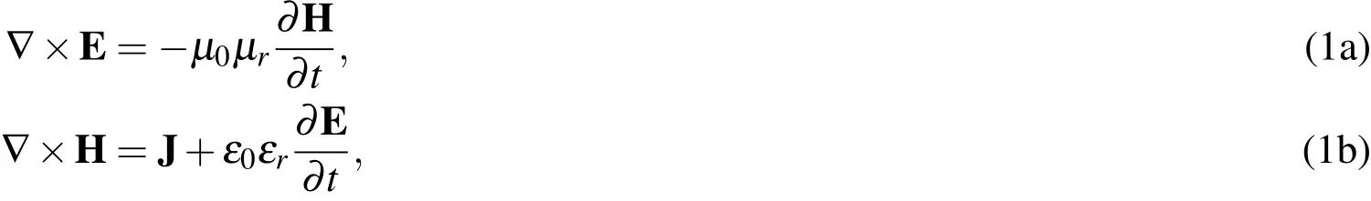
where E and H are the electric and magnetic fields,respectively,J denotes the source,andε0andμ0are the permittivity and permeability offree space,respectively.εrandμrare the relative values of the permittivity and permeability of an actual medium,respectively.

In one dimension,electromagnetic waves traveling in thez-direction,as shown in Fig.1,can be expressed as

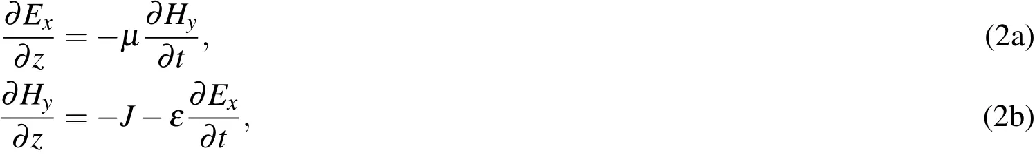
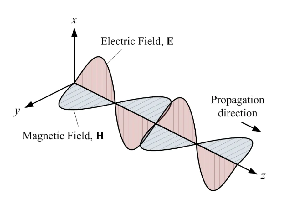
Figure 1:Schematic of plane electromagnetic waves propagating in z-direction

whereEx(z,t)andHy(z,t)are the electric and magnetic fields polarized in thexandy-directions,respectively,with the direction of propagation being in thezdirection.Here,ε(=ε0εr)andμ(=μ0μr)are the permittivity and permeability of the medium,respectively.

Another approach to the analysis of electromagnetic wave propagation is to use second-order vector wave equations for electric and magnetic waves. By combining Eqs.1(a)and 1(b),the Maxwell equations can be rewritten as

Considering a plane electromagnetic wave traveling in thez-direction,Eq.5 can be rewritten as

whereεis assumed to be constant.

3 PML-augmented plane-electromagnetic-wave formulations

3.1 Complex coordinate stretching

To describe the plane electromagnetic waves in unbounded media, a one-dimensional space is considered in which the PMLs are located next to a truncated regular domain,as shown in Fig.2.The regular domain(?regular)and PML(?PML)occupy the?L＜z＜LandL≤|z|＜Ltregions,respectively.It is assumed that conductor boundaries are placed at the outer ends of the PML,such that the electromagnetic fields vanish at both ends.

With reference to Fig.2,a complex coordinate stretching from real(z)to imaginarycoordinates can be de fined as

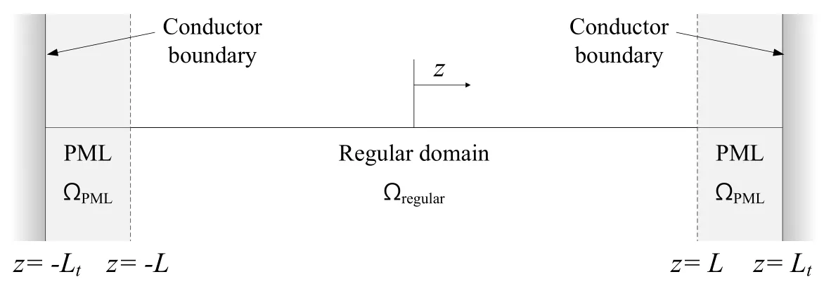
Figure 2:Schematic of PML-truncated computational domain

where ω is the angular frequency,b is the characteristic length of the domain,and crefis the representative wave velocity of the domain.g(s)(=f(s)/b)is an attenuation function that enforces amplitude decay of waves within the PML,but does not affect the wave propagation within the regular domain.Since the coordinate stretching should occur at the PML only,it is expected that g(z)=0 within the regular domain(?L＜z＜L),and g(z)＞0 within the PML(L≤|z|＜Lt).The attenuation functions can be linear,quadratic,cubic,or higher order polynomials,but we choose a cubic function for g(z)in order to obtain satisfactory wave-absorbing performance.Thus,

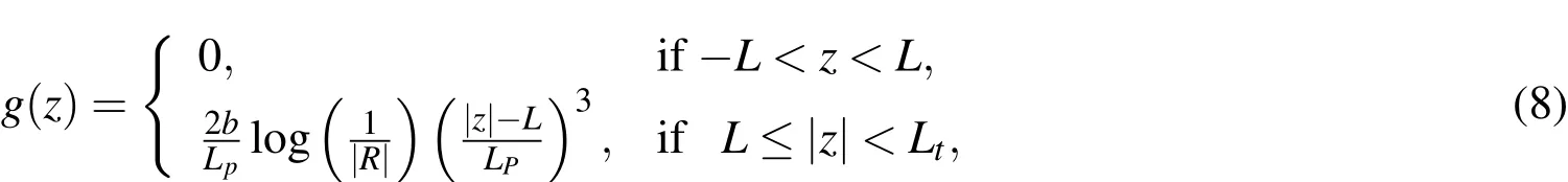
where2L is the length of the regular domain,Lpis the length of the PML,and2Lt(=2L+2LP)is the length of the total domain.R is the complex-valued reflection coefficient that can be tuned to control the amount of reflection from the PML[Kang and Kallivokas(2010)].

3.2 PML-augmented frequency-domain Maxwell equations

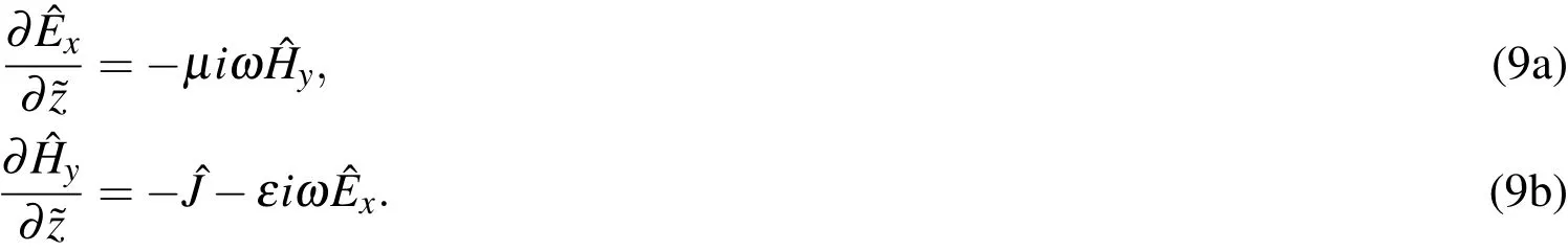
To enforce the attenuation of electromagnetic waves within the PML,the complex coordinate stretching is introduced to the Maxwell equations.Firstly,Eqs.2 are rewritten in terms of the stretched coordinate by replacing the real coordinate z with ?z.Converting the stretched equations into frequency-domain expressions yields

A differential operator can be obtained by differentiating Eq.7 with respect to z,such that

where λ is de fined as in Eq.7,that is,

By applying Eq.10 to Eqs.9(a)and 9(b),these equations can be rewritten as

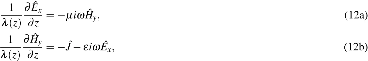
respectively.Multiplying both sides of Eqs.12(a)and 12(b)by λ and iωλ ,respectively,yields

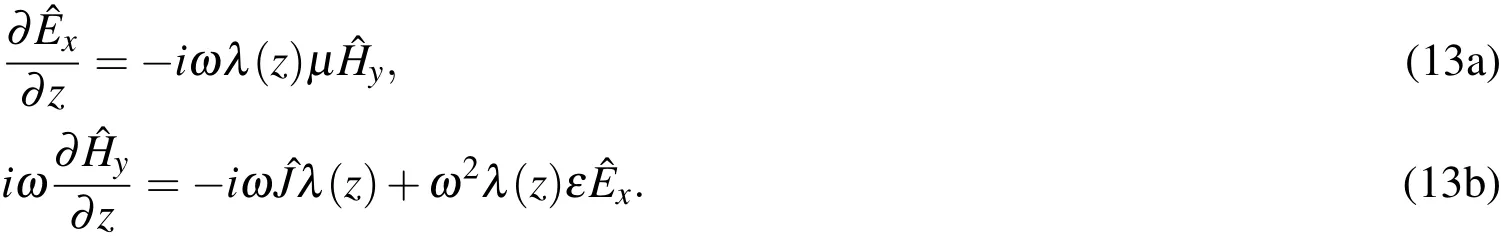
Then,substituting the expression for λ(z)as de fined in Eq.11,the above equations become

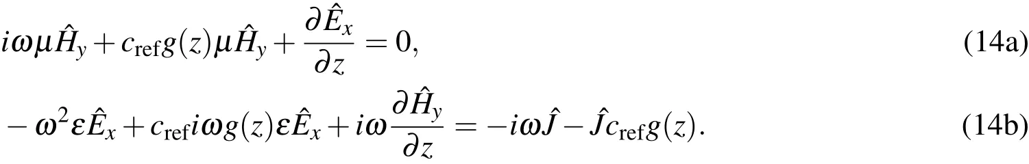
Eqs.14(a)and 14(b)are the PML-augmented Maxwell equations in the frequency domain.

3.3 PML-augmented time-domain Maxwell equations

By applying an inverse Fourier transform to Eqs.14(a)and 14(b),we obtain corresponding PML-augmented equations in the time domain.From these equations,we can establish the following initial boundary value problem(IBVP)in a PML-truncated domain:

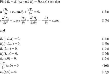
As shown in Fig.2,we set the PML at both ends of the regular domain(?L＜z＜L),and the electric and magnetic fields are 0 at the outer ends of the PML(z=±Lt).Before excitation,no electric and magnetic fields exist in the domain.Then,as the electric charges are accelerated(as expressed by ?J/?t)at the center of the regular domain(z=0),electromagnetic waves are produced that propagate in the±z-direction.

4 Finite element formulations

4.1 Variational formulations

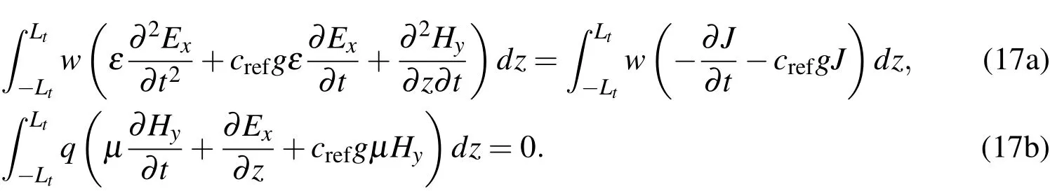
Eqs.15(a)and 15(b)can be cast into variational forms through multiplication by the test functions q(z)and w(z),respectively.Integration over the total domain(?Lt＜z＜Lt)yields

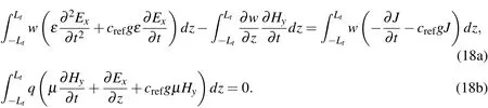
If the last term on the left hand side of Eq.17(a)is integrated by parts and the boundary conditions are applied,the above equations become

4.2 Galerkin finite element formulations

Exand Hycan be approximated as(0,T].These approximations can be introduced using the basis functions φiand ψi,which belong to the same function spaces for each of the electric and magnetic fields,respectively,such that

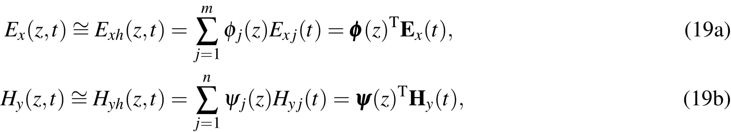
where m and n are the numbers of nodes in which Exand Hyare respectively defined,while φ and ψ are the vectors of φiand ψi,respectively.Exand Hyare column vectors of nodal Exand Hyvalues,respectively.The two functions w(z)and q(z)in Eqs.18 can be approximated as

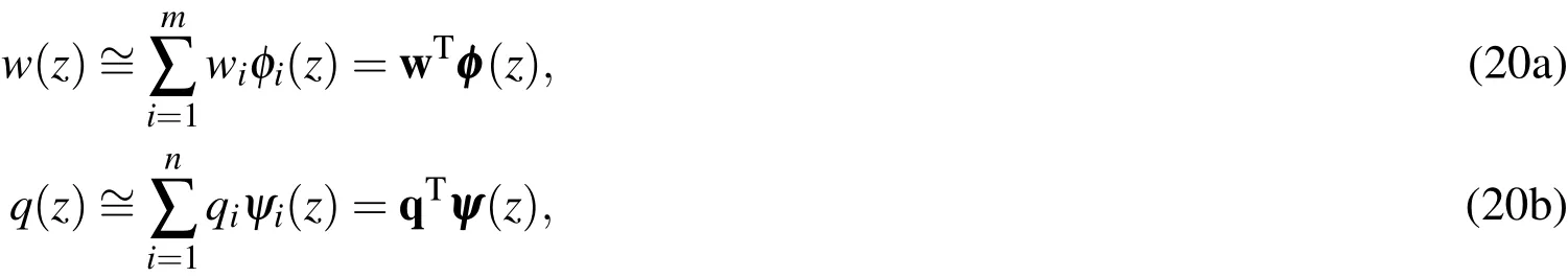
where w and q are vectors of nodal test function values.In mixed finite element methods,the stability of the numerical solutions depends significantly on the polynomial order of the basis functions.In this paper,we used a linear function forφiand a quadratic function forψito obtain stable numerical solutions.Substituting Eqs.19 and 20 into Eqs.18 yields

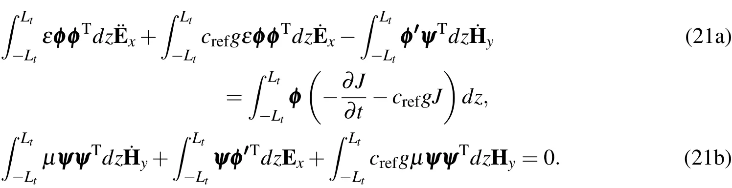
Eqs.21(a)and 21(b)can then be rearranged to form the semi-discrete system of equations

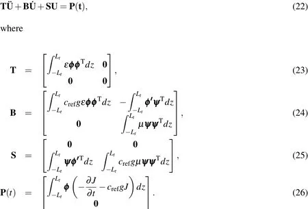
In the above equations,U=[ExHy]Tis a column vector comprising nodal values of the electric and magnetic fields,whereExandHyare treated as independent unknowns.This system of mixed semi-discrete equations can be integrated using direct time-integration schemes such as the Newmark-βmethod.

5 Numerical examples

5.1 Homogeneous domain case

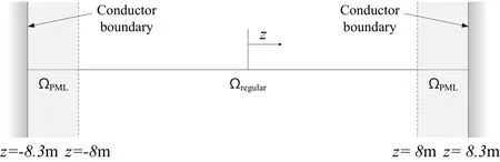
Figure 3:PML-truncated computational domain

To evaluate the PML method suggested in this paper,we considered the PML-truncated one-dimensional domain shown in Fig.3.Here,a 0.3-m PML is attached at z= ±8 m,with εra=1.0059 and μra=1;these values correspond to those of air.|R|=10?14is used for the reflection coefficient.A harmonic current(?J/?t)is excited at the center of the finite domain(z=0).Figs.4(a)and 4(b)show the time history and frequency spectrum of?J/?t,respectively,which is expressed as

Note that?J/?t has 1-GHz frequency.The time step of this example is set to?t=4×10?12s.The element length is Le=0.0025 m,thus,120 elements are present in each PML.The exact solutions of the microwave propagation can be obtained by applying the Laplace transform to Eqs.4 and 6 with the input current given by Eq.27.Thus,

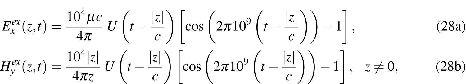
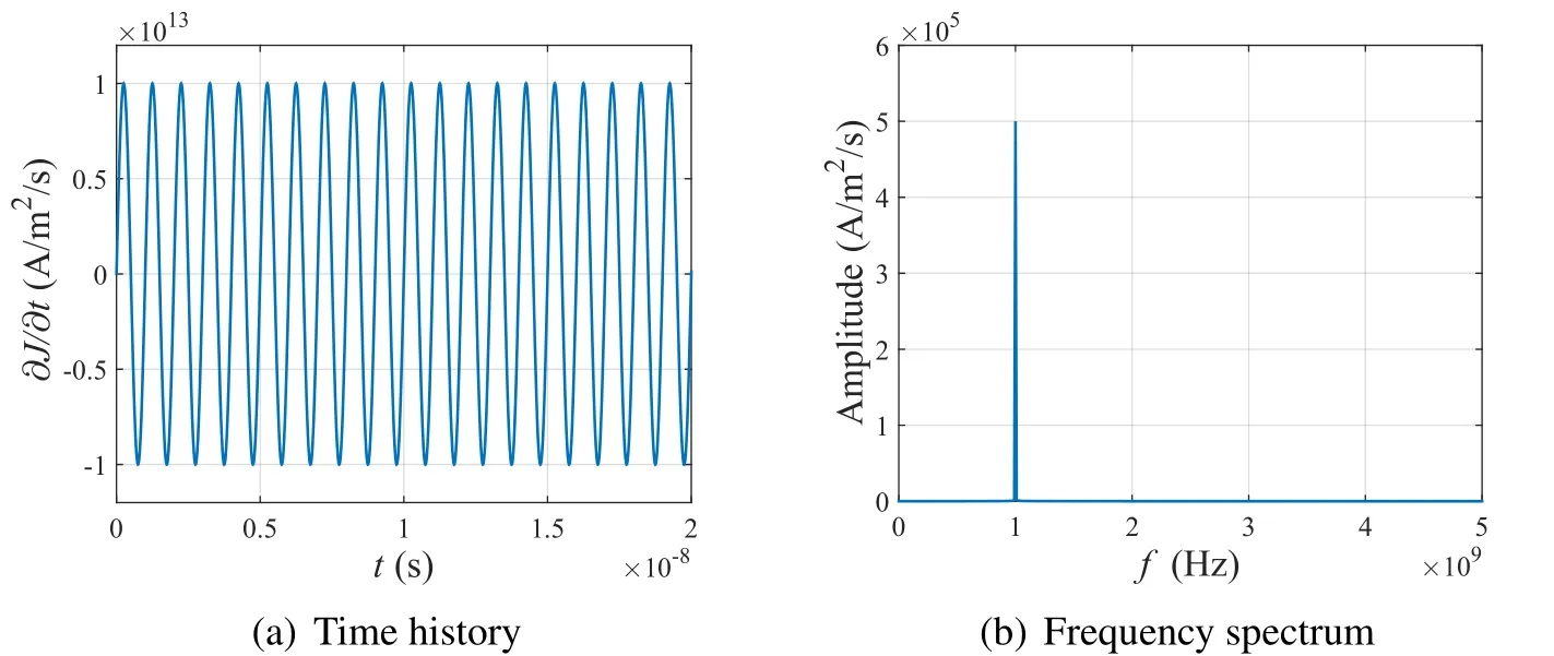
Figure 4:Time history and frequency spectrum of harmonic input current?J/?t

where U(t)is the Heaviside function and c=3×108m/s is the velocity of the electromagnetic waves.Note that there is no exact solution for the magnetic fields at z=0.The propagation shapes of each electric and magnetic wave are shown in Fig.5.Specifically,Figs.5(a)and 5(c)show the distribution of the electric field in the x-direction at t=0.0012μs and t=0.0048μs,respectively,along with the exact solutions for comparison.The electric field is created at the source point and spreads in both the±z-directions.When the electric wave enters the PML,its amplitude decreases without reflection and converges to zero within a few nodes,as illustrated in Fig.5(c).Figs.5(b)and 5(d)show the propagation of the magnetic waves in the z-direction at the same time points as above.The magnetic waves are also created at the center of the regular domain,due to electric charges,and spread in both the±z-directions with opposite sign.Note that,although no exact magnetic wave solution exists at z=0,the numerical solutions pass through the origin.

For the same current source in the same domain,Fig.6 depicts the time history of the electric and magnetic waves at z=1 m.The calculated electric and magnetic fields match the exact solution and no re flected waves are detected.Thus,the mixed finite element method is very applicable to the electromagnetic wave propagation model and the PML attenuates outgoing waves effectively.

To prove the suitability of the suggested method in the multi-frequency case,we considered step-current-pulse excitation.The step current pulse(again modeled by?J/?t)is de fined in Eq.29,while the time history and frequency spectrum of the pulse are depicted in Fig.7.

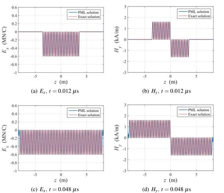
Figure 5:Distribution of Exand Hydue to harmonic current pulse(?J/?t)excitation at midpoint

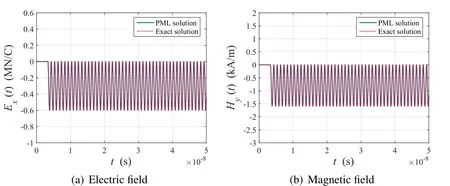
Figure 6:Time history of Exand Hyat z=1 m due to harmonic current pulse(?J/?t)excitation at midpoint

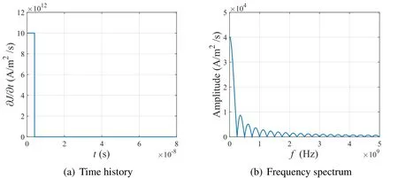
Figure 7:Time history and frequency spectrum of step-pulse input current?J/?t

The exact solutions of the electromagnetic field due to the step current pulse in Eq.29 can be expressed as

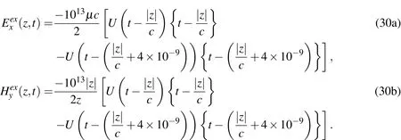
Figs.8 and 9 show the electric and magnetic field responses to the step-pulse excitation.The propagation shapes are illustrated in Fig.8.The numerical solutions match the exact solutions for the electric field well,and the electric and magnetic fields are forced to vanish in the PML.Thus,the PML works effectively for multifrequency excitation as well as single frequency scenarios.However,in the magnetic field case,we can detect nontrivial differences between the exact and numerical solutions at the points immediately adjacent to the source.This is becausez=0 is a singular point in terms of the magnetic field.The numerical solutions capture this singularity by exhibiting spikes near this point.

The time history atz=1 in response to the?J/?tcharge is shown in Fig.9.As the domain is homogeneous,both the electric and magnetic fields remain constant after the current supplement.The numerical solutions conform to the exact solutions.

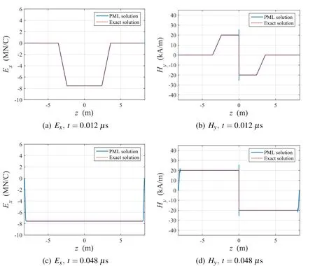
Figure 8:Distribution of Exand Hydue to step current pulse(?J/?t)excitation at midpoint

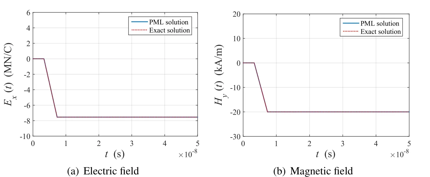
Figure 9:Time history of Exand Hyat z=1 m due to step current pulse(?J/?t)excitation at midpoint

Figure10:ComparisonofL2-norms for numerical and exact solutions in the regular domain 5.2

5.2 Error analysis

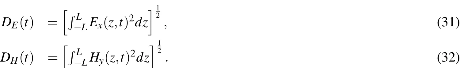
We used the results of the multi-frequency excitation in the homogeneous domain for verification of the developed mixed unsplit- field PML method.We adopted several norms to evaluate the error.First,we introduced theL2-norm,de fined as

Figs.10(a)and 10(b)show theL2-norms of the electric and magnetic fields,respectively,compared with the exact solutions in the regular domain.The calculatedL2-norms conform to the exact solutions.Note that,if the PML were less appropriate in this situation,the calculatedL2-norm would not be constant after the waves entered the PML,because of the effects of the re flected waves.

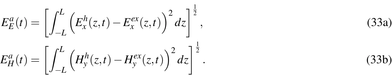
To verify the interrelation between the numerical error and the element lengthLe,we introduced another norm,i.e.,theL2-norm error.This error can be obtained by calculating theL2-norm of the gap between the numerical and exact solutions as

The relationship between theL2-norm errors andLeis illustrated in Fig.11.AsLeis decreased,the error decreases accordingly until a certain critical level is reached.The decrease in theL2-norm error andLeexhibits a linear relation in the log scale.After the critical length limit is reached,further reductions toLeno longer affect the error reduction.In this case,the criticalLefor the error reduction effect were found to be 0.005 m and 0.0025 m for the electric and magnetic fields,respectively.

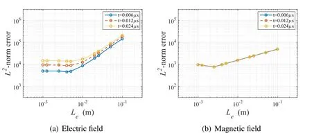
Figure 11:Relationship between Leand L2-norm error

Next,a normalizedL2error was introduced to evaluate the relative error compared to the maximum values of the electric and magnetic fieldL2-norms.This was obtained by normalizing theL2-norm error to the maximum value of theL2-norm of the exact solution,such that

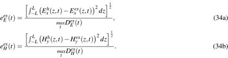
Figure 12:Normalized L2-errors calculated in the regular domain

Fig.12 shows the normalizedL2errors for the electric and magnetic fields.The normalizedL2errors for both fields remain steady after the pulse reaches the PML.Note that,if there were re flections from the PML,the normalizedL2errors would not be constantly maintained as time progressed.Here,the normalizedL2errors were below 0.0005 and 0.01 for the electric and magnetic field solutions,respectively.

An additional error analysis was conducted in relation to the energy metric.The de finition of the electromagnetic energy density is

By integrating Eq.35 over the regular domain,we obtained the total energy in that domain as

Fig.13 illustrates the total energy,the energy associated with the electric field,and the energy associated with the magnetic field.All graphs display the exact solutions for comparison.Note that the instantaneous energy densities associated with the electric and magnetic fields are equal,as predicted by theory.The results are well matched with the energy values calculated from the exact solutions and,as expected,the energy remains constant after the time at which the electromagnetic waves reach the PML.

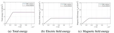
Figure 13:Comparison of energy results for numerical and exact solutions in the regular domain

We also calculated the percentage error for the electric potential.The electric field E and electric potentialVare related according to

In this example,the electric potential can be obtained by integratingExover the regular domain.The calculated electric potential in the regular domain is shown in Fig.14,where the potential is assumed to be zero atz=0.The PML-based results exhibit good agreement with the exact potential.The percentage error based on the electric potential can be de fined as

whereAexandAhrepresent the areas between thez-axis and the calculated electric potential of the exact and PML-endowed electric fields,respectively.For this percentage error,the error due to both a harmonic and a step pulse input current are demonstrated in Fig.15.

Fig.15(a)shows the percentage error of the electric potential due to the harmonic and step pulse excitations expressed in Eq.27and Eq.29,respectively.InFig.15(a),because of the large relative error due to the small initial absolute values of the electric potential,the pattern of the remaining errors is difficult to verify.A magnified graph based on the same result is illustrated in Fig.15(b).Under the harmonic excitation,the percentage error of the electric potential tends to decrease until the wavefronts reach the PML.The waves then exhibit periodic oscillation under approximately 0.03%error.For the step pulse excitation,the error decreases more rapidly than in the previous case,but increases again as the waves propagate.Also,the error magnitude remains stable at 0.05%after entering the PML.

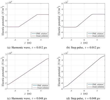
Figure 14:Electric potential distribution according to input current

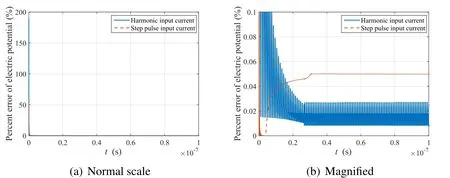
Figure 15:Percentage error based on electric potential

5.3 Heterogeneous domain case

5.3.1 Concrete wall located in domain

To observe the wave transition due to a concrete medium in the domain and for comparison with the homogeneous domain case,we considered a new domain similar to the aforementioned scenario,but in which a concrete wall is located at 4 m≤z≤6.05 m(Fig.16).In this case,εrc=4.5 at the concrete wall andμis the same as in free space.The time step,Le,and other parameters are identical to those of the homogeneous domain case.

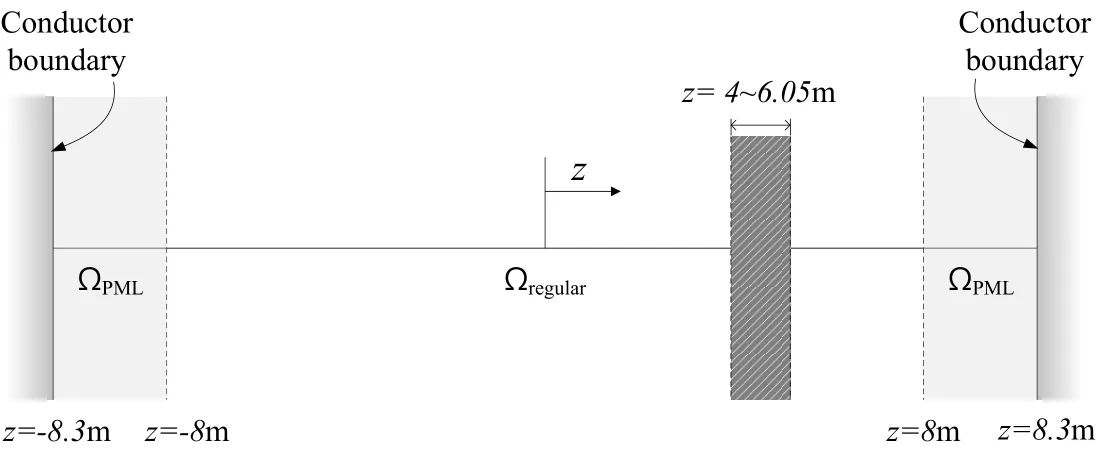
Figure 16:PML-truncated computational domain with a concrete wall between z=4 m and z=6.05 m

The step current pulse of Eq.29 is excited at the center of the PML-truncated one dimensional heterogeneous domain.The corresponding results are illustrated in Figs.17 and 18.Fig.17 shows the distribution of the electric and magnetic fields att=0.0024μs and 0.0048μs.As the waves are transmitted into the concrete wall,the propagating waves are decelerated as a result of the high permittivity.Further,the amplitudes of the electric and magnetic waves vary in opposite directions.When the waves penetrate the concrete wall,the opposite-phase reflected waves appear in the electric field,but the reflected waves in the magnetic field have the same phase as the incident wave.We compared the PML solutions with the solutions of an enlarged domain as an alternative to the in finite domain.The results are shown on the same graphs(Figs.17 and 18).The PML solutions exhibited good agreement with the enlarged domain solutions.

Fig.18 shows the temporal change of the electric and magnetic fields atz=1 m.It is apparent that reverse-and non-reverse-phase reflected waves are detected in the

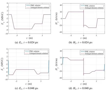
Figure 17:Distribution of Exand Hydue to the step current pulse in the domain containing the concrete wall

electric and magnetic waves,respectively,as in the solution in the enlarged domain.The accuracy of the solutions was quantified using the normalizedL2error based on the enlarged domain solutions,which is de fined as

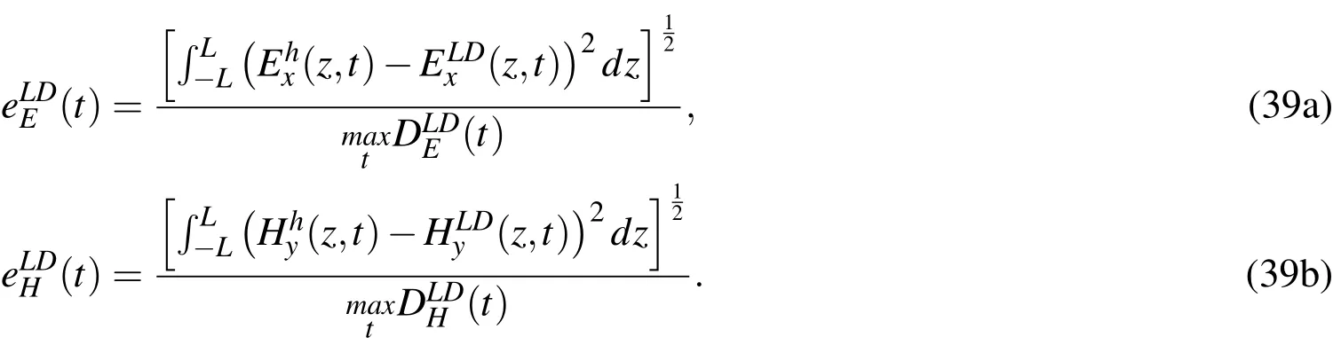
Fig.19 shows the time history of the normalizedL2-error.It is noted that the normalized errors are less than 0.25%for both the electric and magnetic field solutions.

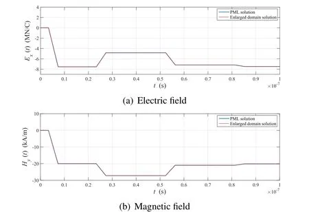
Figure 18:Time history of Exand Hyat z=1 m due to the step current pulse in the domain containing the concrete wall

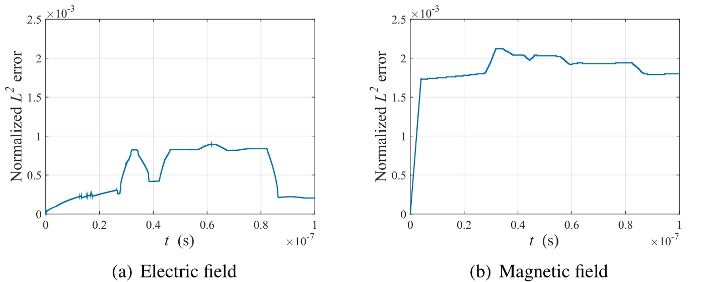
Figure 19:Time history of normalized L2-error in the domain containing the concrete wall

5.3.2 Cracked concrete wall located in domain

To examine additional practical examples,a situation was considered in which a crack was initiated at the center of the concrete wall discussed in the foregoing heterogeneous domain.To create a numerical model of this crack,a space of 5-cm width was evacuated in the center of the concrete wall,as illustrated in Fig.20,and assigned the properties of air.The crack was comprised of twenty numerical elements.

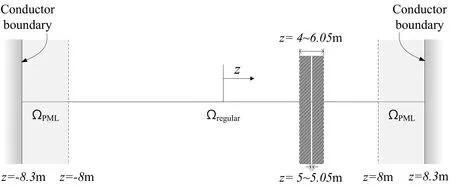
Figure 20:PML-truncated computational domain containing cracked concrete wall

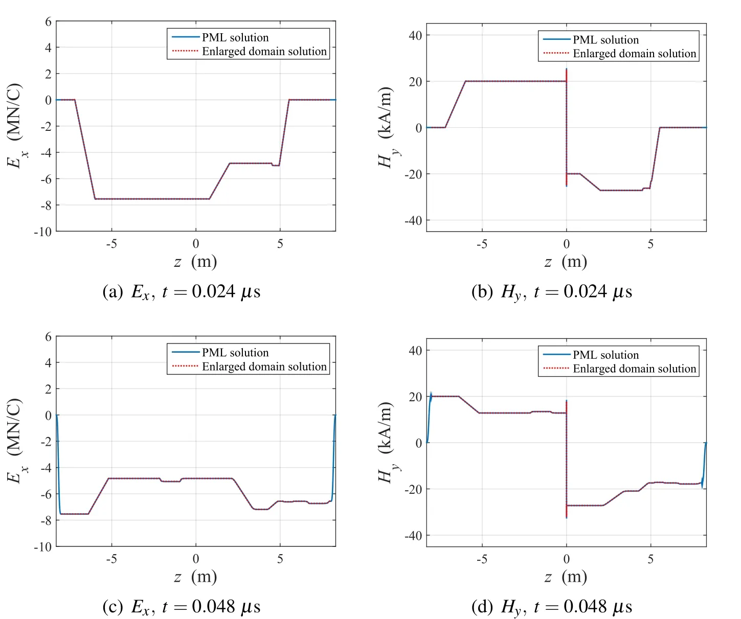
Figure 21:Distribution of Exand Hydue to the step current pulse in the domain containing the cracked concrete wall

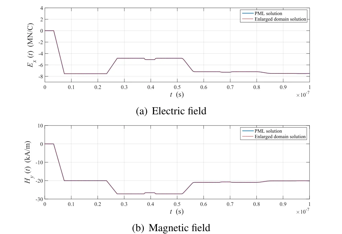
Figure 22:Time history of Exand Hyat z=1 m due to the step current pulse in the domain containing the cracked concrete wall

Figure 23:Time history of normalized L2error in the domain containing the cracked concrete wall

Figs.21 and 22 show the response of the electromagnetic waves to the acceleration of electric charges(described in Eq.29)at the center of the domain.As in the previous case of the uncracked concrete wall,the waves reflected by the concrete were rather flat,as illustrated in Figs.17(c)and 17(d),but in Fig.21 one can easily recognize the shallow sink or protrusion due to the gap inside the concrete wall.The transition is detected in the time history of the electric and magnetic fields perceived atz=1 m,as shown in Fig.22.Also,the same current source is supplied to the same medium in the enlarged domain,and the results are illustrated in Figs.21 and 22 alongside the solutions in the PML-truncated domain.Both results match well in the regular domain.Fig.23 shows the normalizedL2error based on the enlarged domain solutions.As previously,the error is maintained below 0.25%for both field solutions in this case.

6 Conclusion

In this paper,a mixed unsplit- field PML method was developed for the simulation of electromagnetic waves in an unbounded domain.To enforce wave attenuation within the PML,complex coordinate stretching was introduced to the frequencydomain Maxwell equations,and the resulting equations were converted back to the time domain using the inverse Fourier transform.The developed PML-endowed Maxwell equations were solved using a mixed finite element method in the time domain.In particular,the Newmark-βmethod was used for direct time integration of the semi-discrete equations.

In this study,we used linear and quadratic shape functions to approximate the electric and magnetic fields,respectively,in order to obtain stable results for both the electric and magnetic waves.We verified our results using numerical examples of both homogeneous and heterogeneous domains,and showed the excellent waveabsorbing performance of the PML for electromagnetic waves.

The accuracy of the numerical solutions was determined using a series of error analyses.In particular,the normalizedL2error of the electric and magnetic field results for the step current pulse remained at approximately 0.0005 and 0.01,respectively,in the case of a homogeneous domain.Also,we conducted transition simulations in two domains,which contained either an uncracked or a cracked concrete wall,and compared the results to the enlarged domain solutions.We showed the crack resolution performance of the electromagnetic waves using the PML method and obtained satisfactory wave attenuation performance in the PML.The developed PML method may be applied to microwave nondestructive evaluation(NDE)for health monitoring of reinforced concrete(RC)structures.

Acknowledgement:This research was supported by the Basic Science Research Program through the National Research Foundation of Korea(2014R1A1A1006419).

Abarbanel,S.;Gottlieb,D.(1997):A mathematical analysis of the PML method.Journal of Computational Physics,vol.134,pp.357–363.

Bécache,E.;Joly,P.(2002): On the analysis of Berenger’s perfectly matched layers for Maxwell’s equations.Mathematical Modelling and Numerical Analysis,vol.36,pp.87–119.

Bérenger,J.P.(1994): A perfectly matched layer for the absorption of electromagnetic waves.Journal of Computational Physics,vol.114,pp.185–200.

Chew,W.;Liu,Q.(1996):Perfectly matched layers for elastodynamics:A new absorbing boundary condition.Journal of Computational Acoustics,vol.4,pp.341–359.

Drossaert,F.;Giannopoulos,A.(2007):Complex frequency shifted convolution PML for FDTD modelling of elastic waves.Wave Motion,vol.44,pp.593–604.

Jiao,D.;Jin,J.M.;Michielssen,E.;Riley,D.J.(2003): Time-domain finiteelement simulation of three-dimensional scattering and radiation problems using perfectly matched layers.IEEE Transactions on Antennas and Propagation,vol.51,pp.296–305.

Kang,J.W.;Kallivokas,L.F.(2010): Mixed unsplit- field perfectly matched layers for transient simulations of scalar waves in heterogeneous domains.Computational Geosciences,vol.14,no.4,pp.623–648.

Komatitsch,D.;Martin,R.(2007):An unsplit convolutional perfectly matched layer improved at grazing incidence for the seismic wave equation.Geophysics,vol.72,pp.SM155–SM167.

Kucukcoban,S.;Kallivokas,L.F.(2010): A mixed perfectly-matched-layer for transient wave simulations in axisymmetric elastic media.CMES-Computer Modeling in Engineering and Sciences,vol.64,no.2,pp.109–145.

Kuzuoglu,M.;Mittra,R.(1996): Frequency dependence of the constitutive parameters of causal perfectly matched anisotropic absorbers.IEEE Microwave and Guided Wave Letters,vol.6,pp.447–449.

Martin,R.;Komatitsch,D.(2009):An unsplit convolutional perfectly matched layer technique improved at grazing incidence for the viscoelastic wave equation.Geophysical Journal International,vol.179,pp.333–344.

Martin,R.;Komatitsch,D.;Gedney,S.;Bruthiaux,E.(2010):A high-order time and space formulation of the unsplit perfectly matched layer for the seismic wave equation using auxiliary differential equations(ADE-PML).Computer Modeling in Engineering&Sciences,vol.56,pp.17–41.

Roden,J.;Gedney,S.(2000):Convolutional PML(CPML):An efficient FDTD implementation of the CFS-PML for arbitrary media.Microwave and Optical Technology Letters,vol.27,pp.334–339.

Rylander,T.;Jin,J.M.(2005): Perfectly matched layer in three dimensions for the time-domain finite element method applied to radiation problems.IEEE Transactions on Antennas and Propagation,vol.53,pp.1489–1499.

Sagiyama,K.;Govindjee,S.;Persson,P.-O.(2013):An efficient time-domain perfectly matched layers formulation for elastodynamics on spherical domains.Report of the University of California at Berkeley,vol.UCB/SEMM-2013/09.

1Department of Civil&Environmental Engineering,Seoul National University,Seoul,Korea

2Department of Civil Engineering,Hongik University,Seoul,Korea

3Corresponding author E-mail:jwkang@hongik.ac.kr