WEI Ying-san,WANG Yong-sheng

(College of Power Engineering,Naval University of Engineering,Wuhan 430033,China)

1 Introduction

The phenomenon of solution oscillation often occurs at multiple excitation inversion problems[1],and this phenomenon is much more obvious at the low frequency range and the resonance frequencies of the system,which corresponds to low frequency oscillation and resonance oscillation of inversion,respectively[2].In this paper,the multiple excitations on a rectangular plate is estimated by numerical method and analytical method,and the inversion oscillation problem in the excitations estimation process is researched,then some suggestions are put forward to suppress the oscillation and applied on response reconstruction.

2 Virtual experiment design

2.1 Configuration of the experiment

The physical parameters of the plate are as follows:Young’s modulus E=2.07e11 N/m2,Poisson’s ratio ν=0.3,mass density ρ=7 850 kg/m3,damping factor γ=0.03,length（a）×width（b）×thickness（h）=0.6 m×0.5 m×0.001 5 m.On the plate,6 excitation points,9 response points,1 receiving point are configured as ed in Tab.1.In this virtual experiment,4 cases are considered as shown in Tab.2,in which the number of the response points is no less than the number of the excitation points.

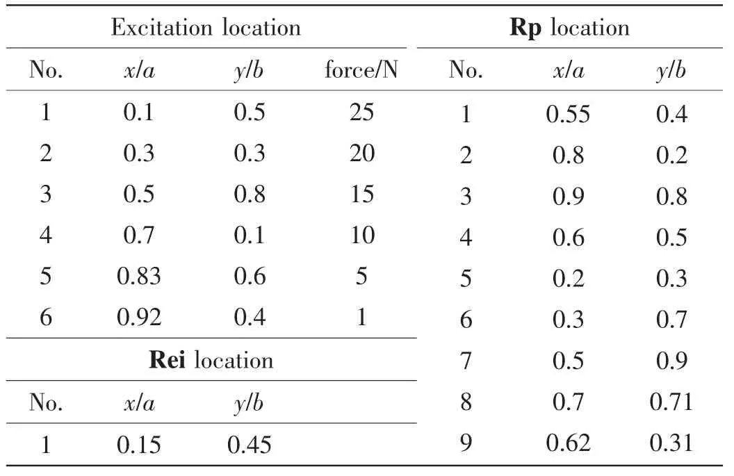
Tab.1 Configuration of the excitation and measured points

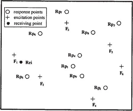
Fig.1 Configuration of the virtual experiment

2.2 Validation

In this part,the mode and response of the plate are calculated by FEM,and the FEM results are compared with the theoretic results,as shown in Fig.2 and Tab.3.The location of the excitation point and response point is(a/2,b/2),(a/4,b/2.5),respectively,and the results agree well,which validates the credibility of the model and method shown in Fig.1.The location of the above points and the magnitude of the excitations are list-

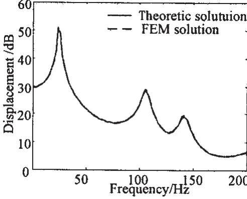
Fig.2 Comparison of displacement responses

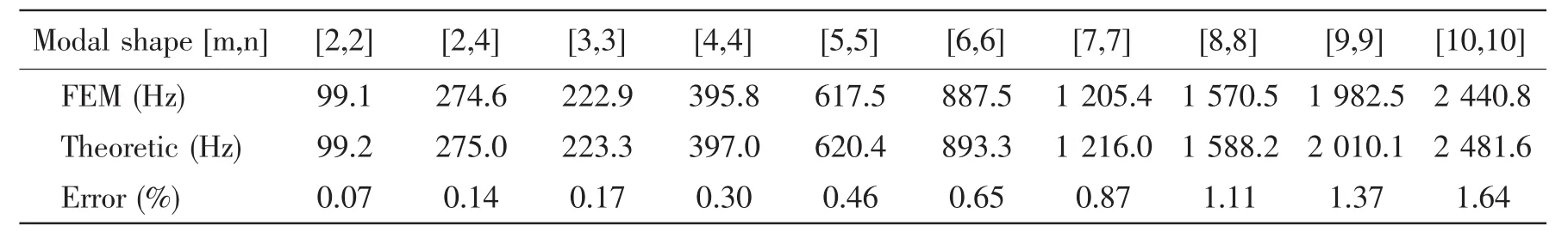
Tab.3 Resonant frequencies of the rectangular plate

3 Multiple excitations inversion of the plate

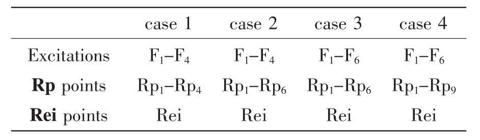
Tab.2 Different experiment schemes

3.1 Construction of acceleration{a?}

Adding the measurement noise to the theoretic acceleration,andis constructed,that:

where ne,nrare the number of excitation points and response points,respectively,and nr≥ne.Niis a normal distributed complex stochastic noise.To ensure the credibility of the result,the vector is constructed with navsamples.

3.2 Construction of accelerances{A?}and{H?}

Fig.3 shown below is a linear system with multiple input and output,and the input X is the multiple excitations on the plate in the simulation,the output Y is the acceleration of the response points.

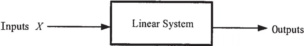
Fig.3 Multi-input and multi-output liner system with samples

The transfer function of the system is:

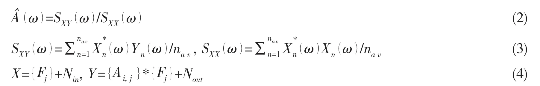
where SXYis the cross spectrum between X and Y,SXXis the power spectrum of X,Nin,Noutare the random noise for the input and output,respectively.From Eq.(4),each element of the transfer matrix can be determined.To estimate the degree of dependence of the input and output signals,the coherence γ is given by

The construction of the matrixcan be determined with the same method.

3.3 Inversion of the excitations

From the above‘measurement’,the acceleration and accelerance data are available which can be adopted to inverse the forces.In this paper,it is assumed that each of the theoretic excitation is constant in the frequency domain and no phase differences are introduced.Then the direct method,TSVD method,Tikhonov regularization method are adopted,respectively,to estimate the forces.By statistic analysis,the excitation samples that lie out of the range of 3σ are rejected.

3.3.1 Inversion by direct method

In the direct method,all singular values of the accelerance are used,and the forces are calculated by the multiplication of pseudo-inverse of accelerance and acceleration

In the low frequency range,the plate modes number is less than the response number,so the accelerance is ill-conditioned,which will result in the inversion oscillation.While in the high frequency range,the oscillation problem is not obvious,as shown in Fig.4,and it shows that:

(1)As the direct method can not improve the ill-condition of the transfer matrix,the solution is oscillation at low frequency range,especially at the plate resonant mode.

(2)When nr＞ne,the transfer matrix is over-determined,and the solution is improved as shown in Cases2 and 4.

(3)In Cases3 and 4,as the magnitude of F6is very small relative to F1-F5,the inversion error is greater than others.

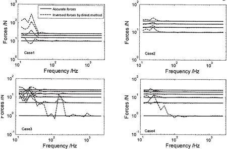
Fig.4 Inversed excitations by direct method

3.3.2 Inversion by TSVD method

The TSVD method only uses a part of singular values of the accelerance.By singular value decomposition,the pseudo-inverse of the accelerance is given by

The key of the TSVD method is how to estimate the threshold value for rejecting of singular values.If the threshold value is too small,then much more small singular values are kept,which will result in system illness.If the value is too big,then much more singular values are rejected,which also will result in solution error,though the ill-condition of the system is improved[1].In this paper,a statistic method is used in the determination of the threshold value,which considers the coherence of the input and output of the system,and the threshold value is dynamically estimated according to the condition number of the system,as shown in Fig.5 from Case1 to Case4.As the transfer matrix is ill-conditioned in low frequency range,so the threshold value has very little effect at high frequency range as shown in Fig.5.According to Ref.[4],an error matrix is defined

where α defines the limits within which thewill fall into Eij.The norm of the error matrix can be used as a threshold to reject the singular values.If all the singular values are less than the error norm then the largest singular value is replaced by error norm itself.Once a pseudo-inverse ofhas been obtained with above considerations,the excitations can be determined

Fig.6 shows the inversed forces by TSVD method.Compared with the result in Fig.4,TSVD method can well improve the low frequency solution oscillation,especially at Case 1 and Case3.

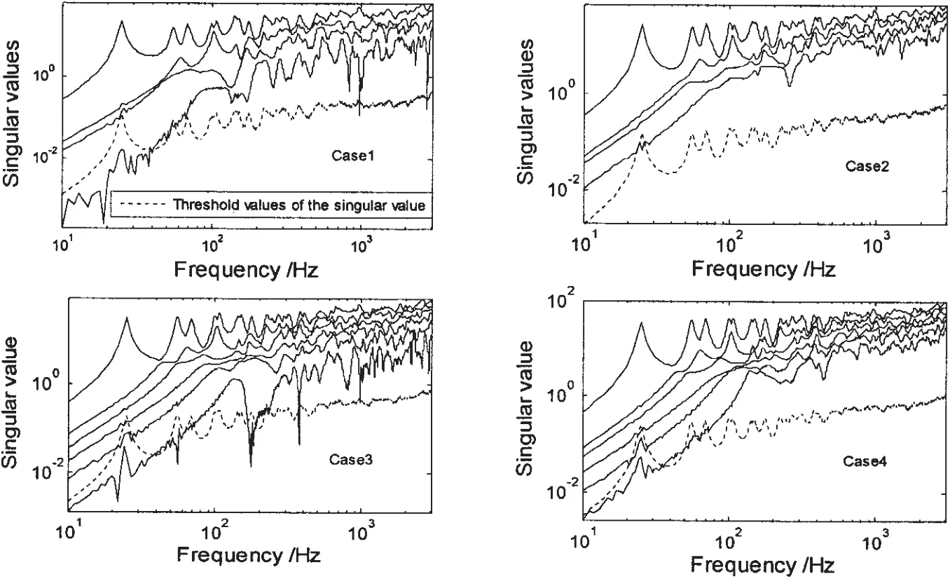
Fig.5 Distribution of the accelerance singular values and the curve of singular value threshold value

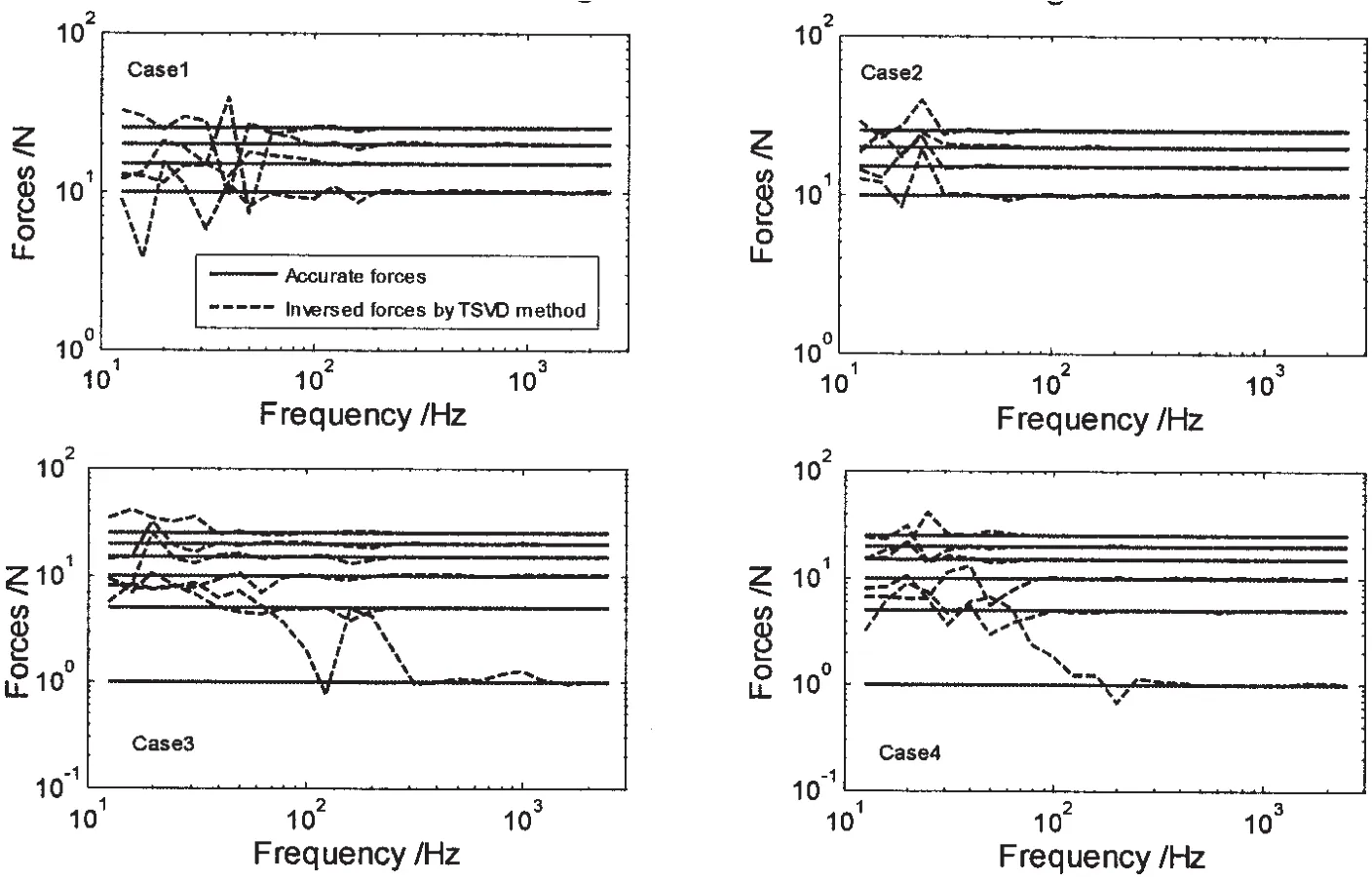
Fig.6 Inversed excitations by TSVD method

3.3.3 Inversion by Tikhonov regularization method

In Tikhonov method,the excitation inversion problem is converted to an optimum problem[1],that:

where ui,viare the vector of the matrixis the filtering factor,which is determined by parameter λ.In the double logarithmic scaling coordinate,the solution norm η and residual norm ρ can be determined with various regularization parameters by Eq.(11).As shown in Fig.7,the curve is a“L”shape,and the optimum λoptis chosen at the corner of the L curve[5],with the maximum curvature at the corner as shown in Fig.8.

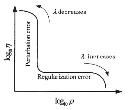
Fig.7 The L curve

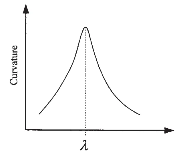
Fig.8 Determination of the optimum regularization parameter

In Fig.7,the horizontal part of the L-curve corresponding to solutions where the regularization error dominates,i.e.at this level of filtering a very smooth solution is produced.In this region the solution is said to be over-regularized because not only noise but also useful information contained in the vectoris suppressed.In the vertical part of the curve insufficient filtering(under-regularization)is applied andis dominated by the effects of noise.Hence,in this region the solution is characterized by many oscillations resulting from higher order singular vectors[5].To balance the regularization error and oscillation error,λoptminimizs both of them.Taking λoptinto Eq.(10),and the optimum excitation vectoris determined.

Herein,the Tikhonov regularization method is used to inverse the excitations in Case1 as an example,as shown in Fig.9.It shows that,the Tikhonov regularization method can well improve the low frequency oscillation problem,while the inversion error increases at the frequency of about 120 Hz,where no oscillation occurs with direct method,and this implies that the solution at 120 Hz is over-regularized,so the optimum regularization factor should be re-calculated.As the excitation inversion problem is frequency dependent,and at each frequency point the optimum regularization factor should be calculated once,which affects the efficiency of this problem.So it is suggested that the Tikhonov regularization method should be adopted at low frequency to improve the low frequency oscillation problem.

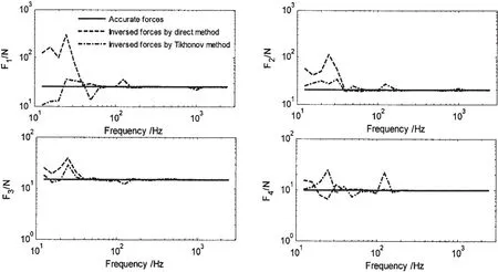
Fig.9 Comparison of inversed excitations by Tikhonov regularization and direct method for Case1

4 Response reconstruction of the receiving point

When the excitations are inversed,the forward problem of the response reconstruction of the receiving point reduces to a simple matrix-vector multiplication.Fig.10 shows the reconstructed response of the receiving point in each case,herein the excitations inversed by Tikhonov method is not used.It can be concluded that,as for direct method,the over-determined transfer matrix can well reconstruct the response as shown in Case2 and Case4,while for TSVD method,all the cases are well reconstructed.

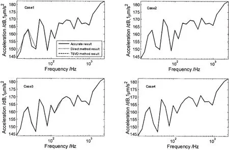
Fig.10 Reconstructed acceleration response of the receiving point

5 Conclusions

To solve the resonance oscillation and low frequency oscillation of the multiple excitation inversion,it is suggested that:(1)Make sure the response points number is greater than the excitation points number to suppress the resonance oscillation;(2)Increase the sample of the measured dates and choose a reasonable threshold value to improve the low frequency oscillation with TSVD method;(3)The Tikhonov regularization method can improve the solution oscillation to some extent in low frequency range,and the regularization parameter should be well chosen.

[1]Visser R.A boundary element approach to acoustic radiation and source identification[D].Ph.D.thesis,University of Twente,2004.

[2]Thite A,Thomopson D.Study of indirect force determination and transfer path analysis using numerical simulations for a flat plate[R].ISVR Technical Memorandum No.851.2000:1-15.

[3]Gorman D J.Free vibration analysis of rectangular plates[M].1st edition.New York:Elsevier,1982.

[4]Janssens M,Verheij J,Thompson D.The use of an equivalent forces method for the experimental quantification of structural sound transmission[J].Journal of Sound and Vibration,1999,226(1):305-328.

[5]Hansen P C.The use of the L-curve in the regularization of discrete ill-posed problems[J].SIAM J Sci.Comput.,1993,14(1):1487-1503.